Mahotas - Watershed

In image processing, a watershed algorithm is used for image segmentation, which is the process of dividing an image into distinct regions. The watershed algorithm is particularly useful for segmenting images with uneven regions or regions with unclear boundaries.

The watershed algorithm is inspired by the concept of a watershed in hydrology, where water flows from high to low areas along ridges until it reaches the lowest points, forming basins.

Similarly, in image processing, the algorithm treats the grayscale values of an image as a topographic surface, where high intensity values represent the peaks and low intensity values represent the valleys.

Working of Watershed Algorithm

Here's a general overview of how the watershed algorithm works in image processing −

Image Preprocessing : Convert the input image to a grayscale image (if it is not in grayscale). Perform any necessary preprocessing steps, such as noise removal or smoothing, to improve the results.
Gradient Calculation : Calculate the gradient of the image to identify the intensity transitions. This can be done by using gradient operators, such as the Sobel operator, to highlight the edges.
Marker Generation : Identify the markers that will be used to initiate the watershed algorithm. These markers generally correspond to the regions of interest in the image.
They can be manually specified by the user or automatically generated based on certain criteria, such as local minima or a clustering algorithm.
Marker Labeling : Label the markers in the image with different integer values, representing different regions.
Watershed Transformation : Calculate the watershed transformation of the image using the labeled markers. This is done by simulating a flooding process, where the intensity values propagate from the markers and fill the image until they meet at the boundaries of different regions.
The result is a grayscale image where the boundaries between regions are highlighted.
Post−processing : The watershed transform may produce over−segmented regions. Post−processing steps, such as merging or smoothing, can be applied to refine the segmentation results and obtain the final segmented image.

Watershed in Mahotas

The Mahotas library does not have a direct function for applying traditional watershed algorithm on an image. However, Mahotas does offer a similar technique called conditional watershed, which we will explore and discuss in more detail in our further chapter.

To have a better understanding on traditional watershed algorithm, let us see an example of performing image segmentation using watershed algorithm with the help of the cv2 library.

Example

In the following example, we are applying Otsu's thresholding, morphological operations, and distance transform to preprocess the image and obtain the foreground and background regions.

We are then using marker−based watershed segmentation to label the regions and mark the boundaries as red in the segmented image.

import cv2
import numpy as np
from matplotlib import pyplot as plt
image = cv2.imread('tree.tiff')
# Convert the image to grayscale
gray = cv2.cvtColor(image, cv2.COLOR_BGR2GRAY)
# Apply Otsu's thresholding
_, thresh = cv2.threshold(gray, 0, 255, cv2.THRESH_BINARY_INV +
cv2.THRESH_OTSU)
# Perform morphological opening for noise removal
kernel = np.ones((3, 3), np.uint8)
opening = cv2.morphologyEx(thresh, cv2.MORPH_OPEN, kernel, iterations=2)
# Perform distance transform
dist_transform = cv2.distanceTransform(opening, cv2.DIST_L2, 5)
# Threshold the distance transform to obtain sure foreground
_, sure_fg = cv2.threshold(dist_transform, 0.7 * dist_transform.max(), 255, 0)
sure_fg = np.uint8(sure_fg)
# Determine the sure background region
sure_bg = cv2.dilate(opening, kernel, iterations=3)
# Determine the unknown region
unknown = cv2.subtract(sure_bg, sure_fg)
# Label the markers for watershed
_, markers = cv2.connectedComponents(sure_fg)
markers = markers + 1
markers[unknown == 255] = 0
# Apply watershed algorithm
markers = cv2.watershed(image, markers)
image[markers == -1] = [255, 0, 0]
# Create a figure with subplots
fig, axes = plt.subplots(1, 2, figsize=(7,5 ))
# Display the original image
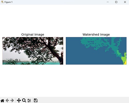
axes[0].imshow(image)
axes[0].set_title('Original Image')
axes[0].axis('off')
# Display the watershed image
axes[1].imshow(markers)
axes[1].set_title('Watershed Image')
axes[1].axis('off')
# Adjust the layout and display the plot
plt.tight_layout()
plt.show()

Output

Following is the output of the above code −

Print Page