Mahotas - SURF Dense Points

SURF (Speeded Up Robust Features) is an algorithm used to detect and describe points of interest in images. These points are called "dense points" or "keypoints" because they are densely present across the image, unlike sparse points which are only found in specific areas.

The SURF algorithm analyzes the entire image at various scales and identifies areas where the intensity changes significantly.

These areas are considered as potential keypoints. They are areas of interest that contain unique and distinctive patterns.

SURF Dense Points in Mahotas

In Mahotas, we use the mahotas.features.surf.dense() function to compute the descriptors at SURF dense points. Descriptors are essentially feature vectors that describe the local characteristics of pixels in an image, such as their intensity gradients and orientations.

To generate these descriptors, the function creates a grid of points across the image, with each point separated by a specific distance. At each point in the grid, an "interest point" is determined.

These interest points are locations where detailed information about the image is captured. Once the interest points are identified, the dense SURF descriptors are computed.

The mahotas.features.surf.dense() function

The mahotas.features.surf.dense() function takes a grayscale image as an input and returns an array containing the descriptors.

This array typically has a structure where each row corresponds to a different interest point, and the columns represent the values of the descriptor features for that point.

Syntax

Following is the basic syntax of the surf.dense() function in mahotas −

mahotas.features.surf.dense(f, spacing, scale={np.sqrt(spacing)},
is_integral=False, include_interest_point=False)

Where,

f − It is the input grayscale image.
spacing − It determines the distance between the adjacent keypoints.
scale (optional) − It specifies the spacing used when computing the descriptors (default is square root of spacing).
is_integral (optional) − It is a flag which indicates whether input image is integer or not (default is 'False').
include_interest_point (optional) − It is also a flag that indicates whether to return the interest points with the SURF points (default is 'False').

Example

In the following example, we are computing the SURF dense points of an image using the mh.features.surf.dense() function.

import mahotas as mh
from mahotas.features import surf
import numpy as np
import matplotlib.pyplot as mtplt
# Loading the image
image = mh.imread('sun.png')
# Converting it to grayscale
image = mh.colors.rgb2gray(image)
# Getting the SURF dense points
surf_dense = surf.dense(image, 120)
# Creating a figure and axes for subplots
fig, axes = mtplt.subplots(1, 2)
# Displaying the original image
axes[0].imshow(image)
axes[0].set_title('Original Image')
axes[0].set_axis_off()
# Displaying the surf dense points
axes[1].imshow(surf_dense)
axes[1].set_title('SURF Dense Point')
axes[1].set_axis_off()
# Adjusting spacing between subplots
mtplt.tight_layout()
# Showing the figures
mtplt.show()

Output

Following is the output of the above code −

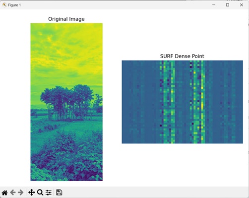
By Adjusting the Scale

We can adjust the scale to compute the descriptors of SURF dense points at different spaces. The scale determines the size of the region that is examined around an interest point.

Smaller scales are good for capturing local details while larger scales are good for capturing global details.

In mahotas, the scale parameter of the surf.dense() function determines the scaling used when computing the descriptors of SURF dense points.

We can pass any value to this parameter to check the impact of scaling on SURF dense points.

Example

In the example mentioned below, we are adjusting the scale to compute descriptors of SURF dense points −

import mahotas as mh
from mahotas.features import surf
import numpy as np
import matplotlib.pyplot as mtplt
# Loading the image
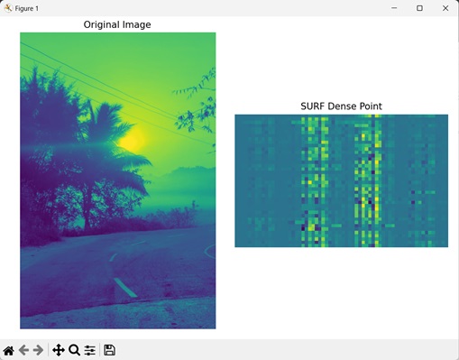
image = mh.imread('nature.jpeg')
# Converting it to grayscale
image = mh.colors.rgb2gray(image)
# Getting the SURF dense points
surf_dense = surf.dense(image, 100, np.sqrt(25))
# Creating a figure and axes for subplots
fig, axes = mtplt.subplots(1, 2)
# Displaying the original image
axes[0].imshow(image)
axes[0].set_title('Original Image')
axes[0].set_axis_off()
# Displaying the surf dense points
axes[1].imshow(surf_dense)
axes[1].set_title('SURF Dense Point')
axes[1].set_axis_off()
# Adjusting spacing between subplots
mtplt.tight_layout()
# Showing the figures
mtplt.show()

Output

Output of the above code is as follows −

By Including Interest Points

We can also include interest points of an image when computing the descriptors of SURF dense points. Interest points are areas where the intensity value of pixels' changes significantly.

In mahotas, to include interest points of an image, we can set the include_interest_point parameter to the boolean value 'True', when computing the descriptors of SURF dense points.

Example

In here, we are including interest points when computing the descriptors of SURF dense points of an image.

import mahotas as mh
from mahotas.features import surf
import numpy as np
import matplotlib.pyplot as mtplt
# Loading the image
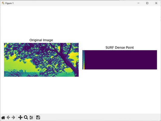
image = mh.imread('tree.tiff')
# Converting it to grayscale
image = mh.colors.rgb2gray(image)
# Getting the SURF dense points
surf_dense = surf.dense(image, 100, include_interest_point=True)
# Creating a figure and axes for subplots
fig, axes = mtplt.subplots(1, 2)
# Displaying the original image
axes[0].imshow(image)
axes[0].set_title('Original Image')
axes[0].set_axis_off()
# Displaying the surf dense points
axes[1].imshow(surf_dense)
axes[1].set_title('SURF Dense Point')
axes[1].set_axis_off()
# Adjusting spacing between subplots
mtplt.tight_layout()
# Showing the figures
mtplt.show()

Output

After executing the above code, we get the following output −

Print Page