Mahotas - Computing Linear Binary Patterns

Linear Binary Patterns (LBP) is used to analyze the patterns in an image. It compares the intensity value of a central pixel in the image with its neighboring pixels, and encodes the results into binary patterns (either 0 or 1).

Imagine you have a grayscale image, where each pixel represents a shade of gray ranging from black to white. LBP divides the image into small regions.

For each region, it looks at the central pixel and compares its brightness with the neighboring pixels.

If a neighboring pixel is brighter or equal to the central pixel, it's assigned a value of 1; otherwise, it's assigned a value of 0. This process is repeated for all the neighboring pixels, creating a binary pattern.

Computing Linear Binary Patterns in Mahotas

In Mahotas, we can use the features.lbp() function to compute linear binary patterns in an image. The function compares the brightness of the central pixel with its neighbors and assigns binary values (0 or 1) based on the comparisons.

These binary values are then combined to create a binary pattern that describes the texture in each region. By doing this for all regions, a histogram is created to count the occurrence of each pattern in the image.

The histogram helps us to understand the distribution of textures in the image.

The mahotas.features.lbp() function

The mahotas.features.lbp() function takes a grayscale image as an input and returns binary value of each pixel. The binary value is then used to create a histogram of the linear binary patterns.

The x−axis of the histogram represents the computed LBP value while the y−axis represents the frequency of the LBP value.

Syntax

Following is the basic syntax of the lbp() function in mahotas −

mahotas.features.lbp(image, radius, points, ignore_zeros=False)

Where,

image − It is the input grayscale image.
radius − It specifies the size of the region considered for comparing pixel intensities.
points − It determines the number of neighboring pixels that should be considered when computing LBP for each pixel.
ignore_zeros (optional) − It is a flag which specifies whether to ignore zero valued pixels (default is false).

Example

In the following example, we are computing linear binary patterns using the mh.features.lbp() function.

import mahotas as mh
import numpy as np
import matplotlib.pyplot as mtplt
# Loading the image
image = mh.imread('nature.jpeg')
# Converting it to grayscale
image = mh.colors.rgb2gray(image)
# Computing linear binary patterns
lbp = mh.features.lbp(image, 5, 5)
# Creating a figure and axes for subplots
fig, axes = mtplt.subplots(1, 2)
# Displaying the original image
axes[0].imshow(image, cmap='gray')
axes[0].set_title('Original Image')
axes[0].set_axis_off()
# Displaying the linear binary patterns
axes[1].hist(lbp)
axes[1].set_title('Linear Binary Patterns')
axes[1].set_xlabel('LBP Value')
axes[1].set_ylabel('Frequency')
# Adjusting spacing between subplots
mtplt.tight_layout()
# Showing the figures
mtplt.show()

Output

Following is the output of the above code −

Ignoring the Zero Valued Pixels

We can ignore the zero valued pixels when computing linear binary patterns. Zero valued pixels are referred to the pixels having an intensity value of 0.

They usually represent the background of an image but may also represent noise. In grayscale images, zero valued pixels are represented by the color 'black'.

In mahotas, we can set the ignore_zeros parameter to the boolean value 'True' to exclude zero valued pixels in the mh.features.lbp() function.

Example

The following example shows computation of linear binary patterns by ignoring the zero valued pixels.

import mahotas as mh
import numpy as np
import matplotlib.pyplot as mtplt
# Loading the image
image = mh.imread('sea.bmp')
# Converting it to grayscale
image = mh.colors.rgb2gray(image)
# Computing linear binary patterns
lbp = mh.features.lbp(image, 20, 10, ignore_zeros=True)
# Creating a figure and axes for subplots
fig, axes = mtplt.subplots(1, 2)
# Displaying the original image
axes[0].imshow(image, cmap='gray')
axes[0].set_title('Original Image')
axes[0].set_axis_off()
# Displaying the linear binary patterns
axes[1].hist(lbp)
axes[1].set_title('Linear Binary Patterns')
axes[1].set_xlabel('LBP Value')
axes[1].set_ylabel('Frequency')
# Adjusting spacing between subplots
mtplt.tight_layout()
# Showing the figures
mtplt.show()

Output

Output of the above code is as follows −

LBP of a Specific Region

We can also compute the linear binary patterns of a specific region in the image. Specific regions refer to a portion of an image having any dimension. It can be obtained by cropping the original image.

In mahotas, to compute linear binary patterns of a specific region, we first need to find the region of interest from the image. To do this, we specify the starting and ending pixel values for the x and y coordinates respectively. Then we can compute the LBP of this region using the lbp() function.

For example, if we specify the values as [300:800], then the region will start from 300 pixels and go up to 800 pixels in the vertical direction (y−axis).

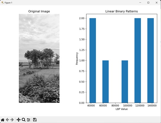
Example

Here, we are computing the LBP of a specific portion of the specified grayscale image.

import mahotas as mh
import numpy as np
import matplotlib.pyplot as mtplt
# Loading the image
image = mh.imread('tree.tiff')
# Converting it to grayscale
image = mh.colors.rgb2gray(image)
# Specifying a region of interest
image = image[300:800]
# Computing linear binary patterns
lbp = mh.features.lbp(image, 20, 10)
# Creating a figure and axes for subplots
fig, axes = mtplt.subplots(1, 2)
# Displaying the original image
axes[0].imshow(image, cmap='gray')
axes[0].set_title('Original Image')
axes[0].set_axis_off()
# Displaying the linear binary patterns
axes[1].hist(lbp)
axes[1].set_title('Linear Binary Patterns')
axes[1].set_xlabel('LBP Value')
axes[1].set_ylabel('Frequency')
# Adjusting spacing between subplots
mtplt.tight_layout()
# Showing the figures
mtplt.show()

Output

After executing the above code, we get the following output −

Print Page