Mahotas - Displaying an Image

---

---

Once you have loaded an image and performed various operations on it, you would need to display the final output image to view the results of your operations.

Displaying an image refers to visually presenting the image data to a user or viewer on a screen.

Displaying an Image in Mahotas

We can display an image in Mahotas using the imshow() and show() functions from the mahotas.plotting module. It allows us to display images within a Python environment. This function internally uses the Matplotlib library to render the image.

Let us discuss about the imshow() and show() function briefly.

Using the imshow() Function

The imshow() function is used to display an image in a separate window. It creates a new window and renders the image within it. This function provides various options to customize the display, such as adjusting the window size, colormap, and color range.

Syntax

Following is the basic syntax of imshow() function −

imshow(image)

Where, 'image' is the picture we want to display.

Using the show() Function

The show() function is used to display the current figure or image. It is a part of the matplotlib library from pylab module, which Mahotas uses for plotting and visualization.

This function is particularly useful when you want to display multiple images or plots in the same window.

Syntax

Following is the basic syntax of show() function −

show()

Example

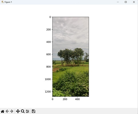
In the following example, we are using the imshow() and show() functions to display an image file named "nature.jpeg" from the current directory −

import mahotas as mh
from pylab import imshow, show
# Loading the image using Mahotas
image = mh.imread('nature.jpeg')
# displaying the original image
imshow(image)
show()

Output

Output of the above code is as follows −

Displaying Multiple Images

Mahotas also allows us to display multiple images simultaneously. This is useful when we want to compare or visualize different images side by side. Mahotas provides a wide range of image formats, including common formats like JPEG, PNG, BMP, TIFF, and GIF. Hence, we can display each image in different formats.

The image formats refer to the different file formats used to store and encode images digitally. Each format has its own specifications, characteristics, and compression methods.

Example

In this example, we demonstrate the versatility of Mahotas by displaying images in different formats using imshow() and show() functions. Each loaded image is stored in a separate variable −

import mahotas as ms
import matplotlib.pyplot as mtplt
# Loading JPEG image
image_jpeg = ms.imread('nature.jpeg')
# Loading PNG image
image_png = ms.imread('sun.png')
# Loading BMP image
image_bmp = ms.imread('sea.bmp')
# Loading TIFF image
image_tiff = ms.imread('tree.tiff')
# Creating a figure and subplots
fig, axes = mtplt.subplots(2, 2)
# Displaying JPEG image
axes[0, 0].imshow(image_jpeg)
axes[0, 0].axis('off')
axes[0, 0].set_title('JPEG Image')
# Displaying PNG image
axes[0, 1].imshow(image_png)
axes[0, 1].axis('off')
axes[0, 1].set_title('PNG Image')
# Displaying BMP image
axes[1, 0].imshow(image_bmp)
axes[1, 0].axis('off')
axes[1, 0].set_title('BMP Image')
# Displaying TIFF image
axes[1, 1].imshow(image_tiff)
axes[1, 1].axis('off')
axes[1, 1].set_title('TIFF Image')
# Adjusting the spacing and layout
mtplt.tight_layout()
# Showing the figure
mtplt.show()

Output

The image displayed is as follows −

Customizing Image Display

When we talk about customizing image display in Mahotas, we are referring to the ability to modify various aspects of how the image is presented on the screen or in a plot. These customizations allow us to enhance the visual representation of the image and provide additional information to the viewer.

Mahotas provides several options for customizing the image display. For instance, we can adjust the colormap, add titles, and modify the display size.

Let us discuss each options for customizing the image display one by one.

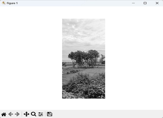
Applying Colormap

Mahotas supports different color maps that can be applied to a grayscale or single−channel images to enhance their contrasts and visual appearance. Color maps determine how pixel values are mapped to colors.

For example, the 'gray' color map is commonly used for grayscale images, while 'hot' or 'jet' color maps can be used to emphasize intensity variations in an image. By choosing an appropriate color map.

To change the colormap used for displaying an image, we can pass the cmap argument to the imshow() function. The cmap argument accepts a string representing the name of the desired colormap.

Example

In the example below, we are passing the cmap argument to the imshow() function and setting it argument to 'gray' to display the grayscale image using a grayscale colormap −

import mahotas as ms
import matplotlib.pyplot as mtplt
# Loading grayscale image
grayscale_image = ms.imread('nature.jpeg', as_grey=True)
# Displaying grayscale image
mtplt.imshow(grayscale_image, cmap='gray')
mtplt.axis('off')
mtplt.show()

Output

After executing the above code, we get the output as shown below −

Adding a Title

We can also add a title or a caption to our image using the title argument passed to the imshow() function.

Example

In the code below, we are adding the title Nature Image' to the displayed image −

import mahotas as ms
import matplotlib.pyplot as mtplt
# Loading the image
image = ms.imread('nature.jpeg')
# Displaying the image
mtplt.imshow(image)
mtplt.axis('off')
mtplt.title('Nature Image')
mtplt.show()

Output

Output of the above code is as follows −

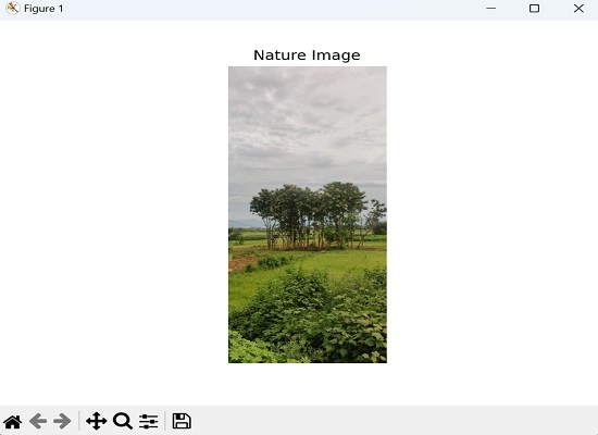
Figure Size

Figure size in mahotas refers to the size of the plot or image display area where the image will be shown.

We can also control the size of the displayed image by specifying the figsize argument of the imshow() function. The figsize argument expects a tuple representing the width and height of the figure in inches.

Example

In the example below, we are setting the figure size to (8, 6) inches −

import mahotas as ms
import matplotlib.pyplot as mtplt
# Loading the image
image = ms.imread('nature.jpeg')
# Set the figure size using Matplotlib
# Specify the width and height of the figure in inches
fig = mtplt.figure(figsize=(8, 6))
# Displaying the image
mtplt.imshow(image)
mtplt.show()

Output

Output of the above code is as follows −