- Mahotas - Home
- Mahotas - Introduction
- Mahotas - Computer Vision
- Mahotas - History
- Mahotas - Features
- Mahotas - Installation
- Mahotas Handling Images
- Mahotas - Handling Images
- Mahotas - Loading an Image
- Mahotas - Loading Image as Grey
- Mahotas - Displaying an Image
- Mahotas - Displaying Shape of an Image
- Mahotas - Saving an Image
- Mahotas - Centre of Mass of an Image
- Mahotas - Convolution of Image
- Mahotas - Creating RGB Image
- Mahotas - Euler Number of an Image
- Mahotas - Fraction of Zeros in an Image
- Mahotas - Getting Image Moments
- Mahotas - Local Maxima in an Image
- Mahotas - Image Ellipse Axes
- Mahotas - Image Stretch RGB
- Mahotas Color-Space Conversion
- Mahotas - Color-Space Conversion
- Mahotas - RGB to Gray Conversion
- Mahotas - RGB to LAB Conversion
- Mahotas - RGB to Sepia
- Mahotas - RGB to XYZ Conversion
- Mahotas - XYZ to LAB Conversion
- Mahotas - XYZ to RGB Conversion
- Mahotas - Increase Gamma Correction
- Mahotas - Stretching Gamma Correction
- Mahotas Labeled Image Functions
- Mahotas - Labeled Image Functions
- Mahotas - Labeling Images
- Mahotas - Filtering Regions
- Mahotas - Border Pixels
- Mahotas - Morphological Operations
- Mahotas - Morphological Operators
- Mahotas - Finding Image Mean
- Mahotas - Cropping an Image
- Mahotas - Eccentricity of an Image
- Mahotas - Overlaying Image
- Mahotas - Roundness of Image
- Mahotas - Resizing an Image
- Mahotas - Histogram of Image
- Mahotas - Dilating an Image
- Mahotas - Eroding Image
- Mahotas - Watershed
- Mahotas - Opening Process on Image
- Mahotas - Closing Process on Image
- Mahotas - Closing Holes in an Image
- Mahotas - Conditional Dilating Image
- Mahotas - Conditional Eroding Image
- Mahotas - Conditional Watershed of Image
- Mahotas - Local Minima in Image
- Mahotas - Regional Maxima of Image
- Mahotas - Regional Minima of Image
- Mahotas - Advanced Concepts
- Mahotas - Image Thresholding
- Mahotas - Setting Threshold
- Mahotas - Soft Threshold
- Mahotas - Bernsen Local Thresholding
- Mahotas - Wavelet Transforms
- Making Image Wavelet Center
- Mahotas - Distance Transform
- Mahotas - Polygon Utilities
- Mahotas - Local Binary Patterns
- Threshold Adjacency Statistics
- Mahotas - Haralic Features
- Weight of Labeled Region
- Mahotas - Zernike Features
- Mahotas - Zernike Moments
- Mahotas - Rank Filter
- Mahotas - 2D Laplacian Filter
- Mahotas - Majority Filter
- Mahotas - Mean Filter
- Mahotas - Median Filter
- Mahotas - Otsu's Method
- Mahotas - Gaussian Filtering
- Mahotas - Hit & Miss Transform
- Mahotas - Labeled Max Array
- Mahotas - Mean Value of Image
- Mahotas - SURF Dense Points
- Mahotas - SURF Integral
- Mahotas - Haar Transform
- Highlighting Image Maxima
- Computing Linear Binary Patterns
- Getting Border of Labels
- Reversing Haar Transform
- Riddler-Calvard Method
- Sizes of Labelled Region
- Mahotas - Template Matching
- Speeded-Up Robust Features
- Removing Bordered Labelled
- Mahotas - Daubechies Wavelet
- Mahotas - Sobel Edge Detection
Mahotas - Haralic Features
Haralick features describes the texture of an image. Texture refers to the patterns in an image that give it a specific look, such as the smoothness of a surface or the arrangement of objects.
To work on Haralick features, we use a special matrix known as gray−level co−occurrence matrix (GLCM). It is a matrix that represents the relationship between pairs of pixel intensities in an image.
It provides information about how frequently different combinations of pixel intensity values occur at specific distances within the image.
Haralic Features in Mahotas
To calculate Haralick features using Mahotas, create the GLCM by specifying the distance and direction of pixel pairs. Next, use the GLCM to calculate various statistical measures that form the Haralick features.
These measures include contrast, correlation, energy, entropy, homogeneity, and more. Finally, retrieve the computed Haralick features.
For example, the contrast feature in Haralick's texture analysis tells us how much the brightness or darkness of neighboring pixels varies in an image. To calculate this feature, we analyze the GLCM matrix.
This matrix shows how often pairs of pixelsx with different brightness levels appear together and where they are located in the image.
We can use the mahotas.features.haralick() function to calculate the haralick features in mahotas.
The mahotas.features.haralick() function
The haralick() function takes a grayscale image as input and returns the calculated Haralick features. Haralick features are calculated based on grayscale images.
Mahotas allows us to calculate Haralick features by analyzing the GLCM of an image. In such way, we can extract information about the texture patterns present in an image.
Syntax
Following is the basic syntax of the haralick() function in mahotas −
mahotas.features.haralick(f, ignore_zeros=False, preserve_haralick_bug=False,
compute_14th_feature=False, return_mean=False, return_mean_ptp=False,
use_x_minus_y_variance=False, distance=1)
Parameters
Following are the parameters accepted by the haralick() function in mahotas −
f − It is the input image.
ignore_zeros (optional) − It computes whether zero values in the input matrix should be ignored (True) or considered (False) when computing the Haralick features.
preserve_haralick_bug (optional) − It determines whether to replicate Haralick's typo in the equations
compute_14th_feature (optional) − It indicates whether to compute the 14th Haralick feature (dissimilarity) or not. By default, it is set to False.
use_x_minus_y_variance (optional) − By default, mahotas uses VAR[P(|x−y|)], but if this parameter is True, it uses VAR[|x−y|].
distance (optional) − It represents the pixel distance used when computing the GLCM. It determines the neighborhood size considered when analyzing the spatial relationship between pixels. By default, it is set to 1.
return_mean − When set to True, the function returns the mean value across all the directions.
return_mean_ptp − When set to True, the function returns the mean value and the point−to−point (ptp) value (difference between max() and min()) across all the directions.
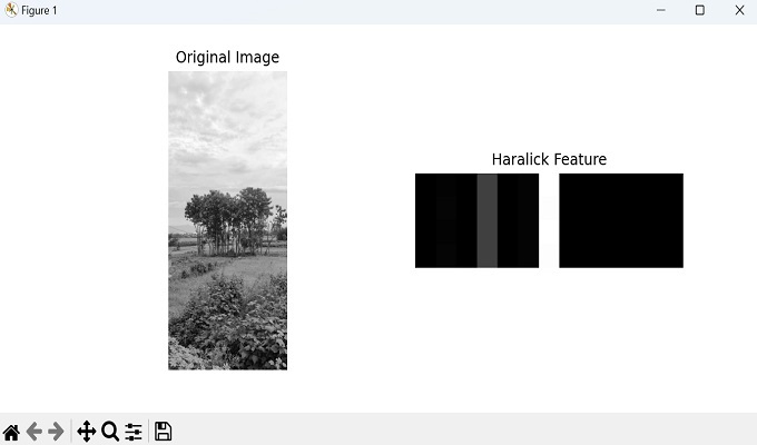
Example
Following is the basic example to calculate the haralic features in mahotas −
import mahotas
import numpy as np
import matplotlib.pyplot as mtplt
# Load a grayscale image
image = mahotas.imread('nature.jpeg', as_grey=True).astype(np.uint8)
# Compute Haralick texture features
features = mahotas.features.haralick(image)
print(features)
# Displaying the original image
fig, axes = mtplt.subplots(1, 2, figsize=(9, 4))
axes[0].imshow(image, cmap='gray')
axes[0].set_title('Original Image')
axes[0].axis('off')
# Displaying the haralick featured image
axes[1].imshow(features, cmap='gray')
axes[1].set_title('Haralick Feature')
axes[1].axis('off')
mtplt.show()
Output
After executing the above code, we get the output as shown below −
[[ 2.77611344e-03  2.12394600e+02  9.75234595e-01  4.28813094e+03
   4.35886838e-01  2.69140151e+02  1.69401291e+04  8.31764345e+00
   1.14305862e+01  6.40277627e-04  4.00793348e+00 -4.61407168e-01
   9.99473205e-01]
 [ 1.61617121e-03  3.54272691e+02  9.58677001e-01  4.28662846e+03
   3.50998369e-01  2.69132899e+02  1.67922411e+04  8.38274113e+00
   1.20062562e+01  4.34549344e-04  4.47398649e+00 -3.83903098e-01
   9.98332575e-01]
 [ 1.92630414e-03  2.30755916e+02  9.73079650e-01  4.28590105e+03
   3.83777866e-01  2.69170823e+02  1.69128483e+04  8.37735303e+00
   1.17467122e+01  5.06580792e-04  4.20197981e+00 -4.18866103e-01
   9.99008620e-01]
 [ 1.61214638e-03  3.78211585e+02  9.55884630e-01  4.28661922e+03
   3.49497239e-01  2.69133049e+02  1.67682653e+04  8.38060403e+00
   1.20309899e+01  4.30756183e-04  4.49912123e+00 -3.80573424e-01
   9.98247930e-01]]
The image displayed is as shown below −
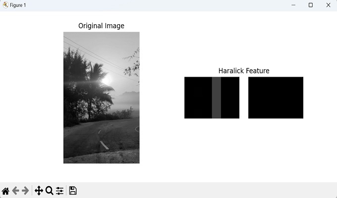
Haralick Features with Ignore Zeros
In certain image analysis scenarios, it is required to ignore specific pixel values during the computation of Haralick texture features.
One common case is when zero values represent a specific background or noise that should be excluded from the analysis.
In Mahotas, we can ignore zero values by setting the ignore_zeros parameter to True.
This will disregard zero values.
Example
In here, we are trying to calculate tha haralicks feature of an image by ignoring its zero values −
import mahotas
import numpy as np
import matplotlib.pyplot as mtplt
# Load a grayscale image
image = mahotas.imread('sun.png', as_grey=True).astype(np.uint8)
# Compute Haralick texture features while ignoring zero pixels
g = ignore_zeros=True
features = mahotas.features.haralick(image,g)
print(features)
# Displaying the original image
fig, axes = mtplt.subplots(1, 2, figsize=(9, 4))
axes[0].imshow(image, cmap='gray')
axes[0].set_title('Original Image')
axes[0].axis('off')
# Displaying the haralick featured image
axes[1].imshow(features, cmap='gray')
axes[1].set_title('Haralick Feature')
axes[1].axis('off')
mtplt.show()
Output
Following is the output of the above code −
[[ 2.67939014e-03   5.27444410e+01 9.94759846e-01  5.03271870e+03
   5.82786178e-01   2.18400839e+02 2.00781303e+04  8.26680366e+00
   1.06263358e+01   1.01107651e-03 2.91875064e+00 -5.66759616e-01
   9.99888025e-01]
 [ 2.00109668e-03   1.00750583e+02 9.89991374e-01  5.03318740e+03
   4.90503673e-01   2.18387049e+02 2.00319990e+04  8.32862989e+00
   1.12183182e+01   7.15118996e-04 3.43564495e+00 -4.86983515e-01
   9.99634586e-01]
 [ 2.29690324e-03   6.34944689e+01 9.93691944e-01  5.03280779e+03
   5.33850851e-01   2.18354256e+02 2.00677367e+04  8.30278737e+00
   1.09228656e+01   8.42614942e-04 3.16166477e+00 -5.26842246e-01
   9.99797686e-01]
 [ 2.00666032e-03   1.07074413e+02 9.89363195e-01  5.03320370e+03
   4.91882840e-01   2.18386605e+02 2.00257404e+04  8.32829316e+00
   1.12259184e+01   7.18459598e-04 3.44609033e+00 -4.85960134e-01
   9.99629000e-01]]
The image obtained is as follows −
Computing Haralick Features with 14th Feature
The 14th feature, Sum of Squares Variance, is calculated as the variance of the GLCM elements weighted by the square of their distances. It provides information about the smoothness of the texture.
A high value indicates a more diverse distribution of pixel pairs in terms of their intensities and distances, indicating a rough texture. Whereas, a low value indicates a more uniform or smooth texture.
In Mahotas, we can compute the Haralicks 14th feature by setting the compute_14th_feature parameter to True.
Example
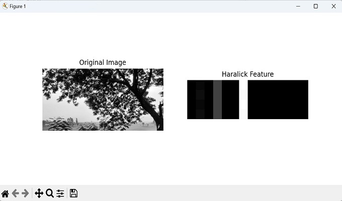
Now, we are computing the 14th haralick features of an image −
import mahotas
import numpy as np
import matplotlib.pyplot as mtplt
# Load a grayscale image
image = mahotas.imread('tree.tiff', as_grey=True).astype(np.uint8)
# Compute Haralick texture features and include the 14th feature
features = mahotas.features.haralick(image, compute_14th_feature=True)
print(features)
# Displaying the original image
fig, axes = mtplt.subplots(1, 2, figsize=(9, 4))
axes[0].imshow(image, cmap='gray')
axes[0].set_title('Original Image')
axes[0].axis('off')
# Displaying the haralick featured image
axes[1].imshow(features, cmap='gray')
axes[1].set_title('Haralick Feature')
axes[1].axis('off')
mtplt.show()
Output
The output produced is as shown below −
[[ 9.21802518e-04  9.60973236e+02  9.37166491e-01  7.64698044e+03
   2.80301553e-01  2.25538844e+02  2.96269485e+04  8.67755638e+00
   1.32391345e+01  2.45576289e-04  5.30868095e+00 -2.86604804e-01
   9.94019510e-01  6.66066209e+00]
 [ 7.16875904e-04  1.64001329e+03  8.92817748e-01  7.65058234e+03
   2.39157134e-01  2.25628036e+02  2.89623161e+04  8.72580856e+00
   1.36201726e+01  1.80965000e-04  5.70631449e+00 -2.37235244e-01
   9.87128410e-01  6.52870916e+00]
 [ 8.28978095e-04  9.93880455e+02  9.35041963e-01  7.65017308e+03
   2.64905787e-01  2.25647417e+02  2.96068119e+04  8.69690646e+00
   1.33344285e+01  2.21103895e-04  5.38241896e+00 -2.74238405e-01
   9.92754897e-01  7.00379254e+00]
 [ 7.11697171e-04  1.51531034e+03  9.00967635e-01  7.65058141e+03
   2.38821560e-01  2.25628110e+02  2.90870153e+04  8.72404507e+00
   1.35861240e+01  1.82002747e-04  5.66026317e+00 -2.41641969e-01
   9.87980919e-01  6.65491250e+00]]
We get the image as follow −