Mahotas - RGB to Sepia

Sepia refers to a special coloring effect that makes a picture look old−fashioned and warm.

When you see a sepia−toned photo, it appears to have a reddish−brown tint. It's like looking at an image through a nostalgic filter that gives it a vintage vibe.

To convert an RGB image to sepia, you need to transform the red, green, and blue color channels of each pixel to achieve the desired sepia tone.

RGB to Sepia Conversion in Mahotas

In Mahotas, we can convert an RGB image to sepia−toned image using the colors.rgb2sepia() function.

To understand the conversion, let's start with the RGB color model −

In RGB, an image is made up of three primary colors− red, green, and blue.
Each pixel in the image has a value for these three colors, which determines its overall color. For example, if a pixel has high red and low green and blue values, it will appear as a shade of red.
Now, to convert an RGB image to Sepia using mahotas, we follow a specific formula. The formula involves calculating new values for the red, green, and blue channels of each pixel.
These new values create the Sepia effect by giving the image a warm, brownish tone.

RGB to Sepia Conversion Steps

Here's a simple explanation of the conversion process −

Start with an RGB image − An RGB image is composed of three color channels− red, green, and blue. Each pixel in the image has intensity values for these three channels, ranging from 0 to 255.
Calculate the intensity of each pixel − To convert to sepia, we first need to calculate the overall intensity of each pixel. This can be done by taking a weighted average of the red, green, and blue color channels.
The weights used in the average can be different depending on the desired sepia effect.
Adjust the intensity values − Once we have the intensity values, we can apply some specific transformations to obtain the sepia effect. These transformations involve adjusting the levels of red, green, and blue channels in a way that mimics the sepia tone.
This can be done by increasing the red channel's intensity, decreasing the blue channel's intensity, and keeping the green channel relatively unchanged.
Clip the intensity values − After the adjustments, some intensity values may go beyond the valid range (0 to 255 for 8−bit images).To ensure the values stay within this range, we need to clip them.
Values below 0 are set to 0, and values above 255 are set to 255.
Reconstruct the sepia image − Finally, the adjusted intensity values are used to reconstruct the sepia image. The image now appears with the desired sepia tone, giving it a vintage look.

Using the mahotas.colors.rgb2sepia() Function

The mahotas.colors.rgb2sepia() function takes an RGB image as input and returns the sepia version of the image.

The resulting sepia image retains the overall structure and content of the original RGB image but introduces a warm, brownish tone.

Syntax

Following is the basic syntax of the rgb2sepia() function in mahotas −

mahotas.colors.rgb2sepia(rgb)

where, rgb is the input image in RGB color space.

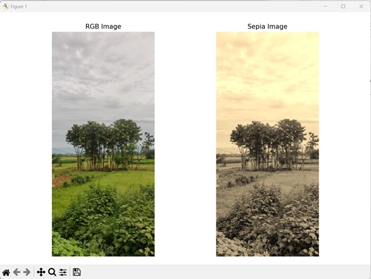
Example

In the following example, we are converting an RGB image to a sepia image using the mh.colors.rgb2sepia() function −

import mahotas as mh
import numpy as np
import matplotlib.pyplot as mtplt
# Loading the image
image = mh.imread('nature.jpeg')
# Converting it to Sepia
sepia_image = mh.colors.rgb2sepia(image)
# Creating a figure and axes for subplots
fig, axes = mtplt.subplots(1, 2)
# Displaying the original RGB image
axes[0].imshow(image)
axes[0].set_title('RGB Image')
axes[0].set_axis_off()
# Displaying the sepia image
axes[1].imshow(sepia_image)
axes[1].set_title('Sepia Image')
axes[1].set_axis_off()
# Adjusting spacing between subplots
mtplt.tight_layout()
# Showing the figures
mtplt.show()

Output

Following is the output of the above code −

Using Transformation Factor

Another approach we can use to convert an RGB to sepia is by adjusting the intensities of each color channel using predetermined coefficients, which are based on the contribution of each channel to the final sepia image.

The contribution of each channel to sepia is calculated as follows −

TR = 0.393 * R + 0.769 * G + 0.189 * B
TG = 0.349 * R + 0.686 * G + 0.168 * B
TB = 0.272 * R + 0.534 * G + 0.131 * B

where TR, TG and TB are the transformation factors of red, green, and blue respectively.

Applying these transformations to each pixel in the RGB image results in the entire sepiatoned image.

Example

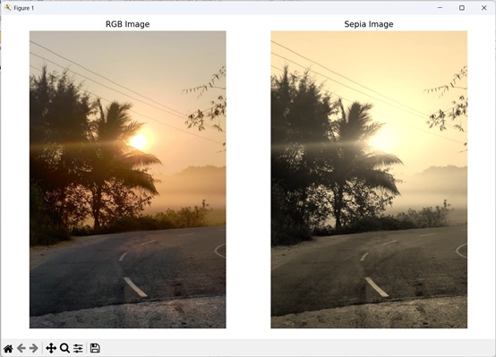
The following example shows conversion of an RGB image to sepia using transformation factors of the RGB channels −

import mahotas as mh
import numpy as np
import matplotlib.pyplot as plt
# Loading the image
image = mh.imread('sun.png')
# Getting the dimensions of the image
height, width, _ = image.shape
# Converting it to Sepia
# Creating an empty array for the sepia image
sepia_image = np.empty_like(image)
for y in range(height):
   for x in range(width):
      # Geting the RGB values of the pixel
      r, g, b = image[y, x]
      # Calculating tr, tg, tb
      tr = int(0.393 * r + 0.769 * g + 0.189 * b)
      tg = int(0.349 * r + 0.686 * g + 0.168 * b)
      tb = int(0.272 * r + 0.534 * g + 0.131 * b)
      # Normalizing the values if necessary
      if tr > 255:
         tr = 255
      if tg > 255:
         tg = 255
      if tb > 255:
         tb = 255
      # Setting the new RGB values in the sepia image array
      sepia_image[y, x] = [tr, tg, tb]
# Creating a figure and axes for subplots
fig, axes = plt.subplots(1, 2)
# Displaying the original RGB image
axes[0].imshow(image)
axes[0].set_title('RGB Image')
axes[0].set_axis_off()
# Displaying the sepia image
axes[1].imshow(sepia_image)
axes[1].set_title('Sepia Image')
axes[1].set_axis_off()
# Adjusting spacing between subplots
plt.tight_layout()
# Showing the figures
plt.show()

Output

Output of the above code is as follows −

Print Page