Mahotas - Mean Filter

The mean filter is used to smooth out an image to reduce noise. It works by calculating the average value of all the pixels within a specified neighborhood and then, replaces the value of the original pixel with the average value.

Let's imagine we have a grayscale image with varying intensity values. Hence, some pixels may have a higher intensity value than other pixels.

Thus, the mean filter is used to create a uniform appearance of the pixels by slightly blurring the image.

Mean Filter in Mahotas

To apply the mean filter in mahotas, we can use the mean_filter() function.

The mean filter in Mahotas uses a structuring element to examine pixels in a neighborhood.

The structuring element replaces each value of pixel with the average value of its neighbouring pixels.

The size of the structuring element determines the extent of smoothing. A larger neighborhood results in stronger smoothing effect, while reducing some finer details, whereas a smaller neightborhood results in less smoothing but maintains more details.

The mahotas.mean_filter() function

The mean_filter() function applies the mean filter to the input image using the specified neighborhood size.

It replaces each pixel value with the majority value among its neighbors. The filtered image is stored in the output array.

Syntax

Following is the basic syntax of the mean filter() function in mahotas −

mahotas.mean_filter(f, Bc, mode='ignore', cval=0.0, out=None)

Where,

img − It is the input image.
Bc − It is the structuring element that defines the neighbourhood.
mode (optional) − It specifies how the function handles the borders of the image. It can take different values such as 'reflect', 'constant', 'nearest', 'mirror' or 'wrap'.
By default, it is set to 'ignore', which means the filter ignores pixels beyond the image's borders.
cval (optional) − The value to be used when mode='constant'. The default value is 0.0.
out (optional) − It specifies the output array where the filtered image will be stored. It must be of the same shape as the input image.

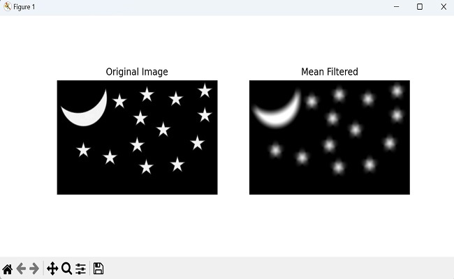
Example

Following is the basic example to filter the image using the mean_filter() function −

import mahotas as mh
import numpy as np
import matplotlib.pyplot as mtplt
image=mh.imread('tree.tiff', as_grey = True)
structuring_element = mh.disk(12)
filtered_image = mh.mean_filter(image, structuring_element)
# Displaying the original image
fig, axes = mtplt.subplots(1, 2, figsize=(9, 4))
axes[0].imshow(image, cmap='gray')
axes[0].set_title('Original Image')
axes[0].axis('off')
# Displaying the mean filtered image
axes[1].imshow(filtered_image, cmap='gray')
axes[1].set_title('Mean Filtered')
axes[1].axis('off')
mtplt.show()

Output

After executing the above code, we get the following output −

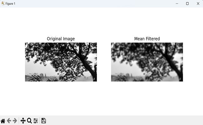
Mean Filter with Reflect Mode

When we apply the mean filter to an image, we need to consider the neighboring pixels around each pixel to calculate the average. However, at the edges of the image, there are pixels that don't have neighbors on one or more sides.

To address this issue, we use the 'reflect' mode. Reflect mode creates a mirror−like effect along the edges of the image. It allows us to virtually extend the image by duplicating its pixels in a mirrored manner.

This way, we can provide the mean filter with neighboring pixels even at the edges.

By reflecting the image values, the mean filter can now consider these mirrored pixels as if they were real neighbors.

It calculates the average value using these virtual neighbors, resulting in a more accurate smoothing process at the image edges.

Example

In here, we are trying to calculate the mean filter with the reflect mode −

import mahotas as mh
import numpy as np
import matplotlib.pyplot as mtplt
image=mh.imread('nature.jpeg', as_grey = True)
structuring_element = mh.morph.dilate(mh.disk(12), Bc=mh.disk(12))
filtered_image = mh.mean_filter(image, structuring_element, mode='reflect')
# Displaying the original image
fig, axes = mtplt.subplots(1, 2, figsize=(9, 4))
axes[0].imshow(image, cmap='gray')
axes[0].set_title('Original Image')
axes[0].axis('off')
# Displaying the mean filtered image
axes[1].imshow(filtered_image, cmap='gray')
axes[1].set_title('Mean Filtered')
axes[1].axis('off')
mtplt.show()

Output

Output of the above code is as follows −

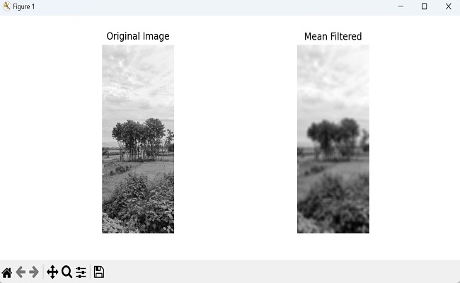
By Storing Result in an Output Array

We can store the result of the mean filter in an output array as well using Mahotas. To achieve this, we first need to create an empty array using the NumPy library.

This array is initialized with the same shape as the input image to store the resultant filtered image. The data type of the array is specified as float (default).

Finally, we store the resultant filtered image in the output array by passing it as a parameter to the mean_filter() function.

Example

Now, we are trying to apply mean filter to a grayscale image and store the result in a specific output array −

import mahotas as mh
import numpy as np
import matplotlib.pyplot as mtplt
image=mh.imread('pic.jpg', as_grey = True)
# Create an output array for the filtered image
output = np.empty(image.shape)
# store the result in the output array
mh.mean_filter(image, Bc=mh.disk(12), out=output)
# Displaying the original image
fig, axes = mtplt.subplots(1, 2, figsize=(9, 4))
axes[0].imshow(image, cmap='gray')
axes[0].set_title('Original Image')
axes[0].axis('off')
# Displaying the mean filtered image
axes[1].imshow(output, cmap='gray')
axes[1].set_title('Mean Filtered')
axes[1].axis('off')
mtplt.show()

Output

Following is the output of the above code −

Print Page