Mahotas - Getting Border of Labels

---

---

Getting the border of labels refers to extracting the border pixels of a labeled image. A border can be defined as a region whose pixels are located at the edges of an image. A border represents the transition between different regions of an image.

Getting borders of labels involves identifying the border regions in the labeled image and separating them from the background.

Since a labeled image consists of only the foreground pixels and the background pixels, the borders can be easily identified as they are present adjacent to the background regions.

Getting Border of labels in Mahotas

In Mahotas, we can use the mahotas.labeled.borders() function to get the border of labels. It analyzes the neighboring pixels of the labeled image and considers the connectivity patterns to get the borders.

The mahotas.labeled.borders() function

The mahotas.labeled.borders() function takes a labeled image as input and returns an image with the highlighted borders.

In the resultant image, the border pixels have a value of 1 and are part of the foreground.

Syntax

Following is the basic syntax of the borders() function in mahotas −

mahotas.labeled.borders(labeled, Bc={3x3 cross}, out={np.zeros(labeled.shape,
bool)})

Where,

• labeled − It is the input labeled image.

• Bc (optional) − It is the structuring element used for connectivity.

• out (optional) − It is the output array (defaults to new array of same shape as labeled).

Example

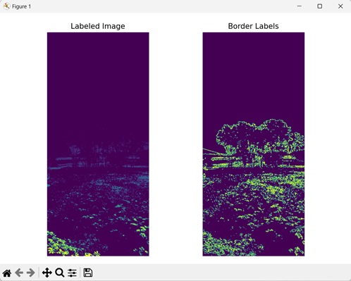
In the following example, we are getting the borders of labels using the mh.labeled.borders() function.

import mahotas as mh
import numpy as np
import matplotlib.pyplot as mtplt
# Loading the image
image = mh.imread('nature.jpeg', as_grey=True)
# Applying thresholding
image = image > image.mean()
# Converting it to a labeled image
labeled, num_objects = mh.label(image)
# Geting border of labels
borders = mh.labeled.borders(labeled)
# Creating a figure and axes for subplots
fig, axes = mtplt.subplots(1, 2)
# Displaying the labeled image
axes[0].imshow(labeled)
axes[0].set_title('Labeled Image')
axes[0].set_axis_off()
# Displaying the borders
axes[1].imshow(borders)
axes[1].set_title('Border Labels')
axes[1].set_axis_off()
# Adjusting spacing between subplots
mtplt.tight_layout()
# Showing the figures
mtplt.show()

Output

Following is the output of the above code −

Getting Borders by using a Custom Structuring Element

We can also get borders of labels by using a custom structuring element. A structuring element is an array which consists of only 1s and 0s. It is used to define the connectivity structure of the neighboring pixels.

Pixels that are included in the connectivity analysis have the value 1, while the pixels that are excluded have the value 0.

In mahotas, we create a custom structuring element using the mh.disk() function. Then, we set this custom structuring element as the Bc parameter in the borders() function to get the borders of labels.

Example

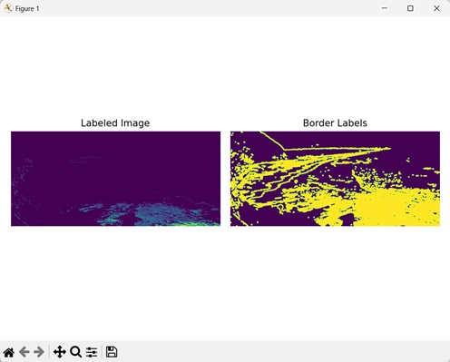
Here, we are getting borders of labels using a custom structuring element.

import mahotas as mh
import numpy as np
import matplotlib.pyplot as mtplt
# Loading the image
image = mh.imread('sea.bmp', as_grey=True)
# Applying thresholding
image = image > image.mean()
# Converting it to a labeled image
labeled, num_objects = mh.label(image)
# Geting border of labels
borders = mh.labeled.borders(labeled, mh.disk(5))
# Creating a figure and axes for subplots
fig, axes = mtplt.subplots(1, 2)
# Displaying the labeled image
axes[0].imshow(labeled)
axes[0].set_title('Labeled Image')
axes[0].set_axis_off()
# Displaying the borders
axes[1].imshow(borders)
axes[1].set_title('Border Labels')
axes[1].set_axis_off()
# Adjusting spacing between subplots
mtplt.tight_layout()
# Showing the figures
mtplt.show()

Output

Output of the above code is as follows −