Mahotas - Regional Minima of Image

Regional minima in an image refer to a point where the intensity value of pixels is the lowest. In an image, regions which form the regional minima are the darkest amongst all other regions. Regional minima are also known as global minima.

Regional minima consider the entire image, while local minima only consider a local neighborhood, to find the pixels with lowest intensity.

Regional minima are a subset of local minima, so all regional minima are a local minima but not all local minima are regional minima.

An image can contain multiple regional minima but all regional minima will be of equal intensity. This happens because only the lowest intensity value is considered for regional minima.

Regional Minima of Image in Mahotas

In Mahotas, we can use the mahotas.regmin() function to find the regional maxima in an image. Regional minima are identified through intensity valleys within an image because they represent low intensity regions.

The regional minima points are highlighted as white against black background, which represents normal points.

The mahotas.regmin() function

The mahotas.regmax() function gets regional minima from an input grayscale image. It outputs an image where the 1's represent presence of regional minima points and 0's represent normal points.

The regmin() function uses a morphological reconstruction−based approach to find the regional minima. Here, the intensity value of each local minima region is compared with its neighboring local minima regions.

If a neighbor is found to have a lower intensity, it becomes the new regional minima. This process continues until no region of lower intensity is left, indicating that the regional minima has been identified.

Syntax

Following is the basic syntax of the regmin() function in mahotas −

mahotas.regmin(f, Bc={3×3 cross}, out={np.empty(f.shape, bool)})

Where,

f − It is the input grayscale image.
Bc (optional) − It is the structuring element used for connectivity.
out(optional) − It is the output array of Boolean data type (defaults to new array of same size as f).

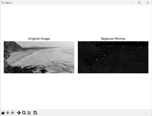
Example

In the following example, we are getting the regional minima of an image using mh.regmin() function.

import mahotas as mh
import numpy as np
import matplotlib.pyplot as mtplt
# Loading the image
image = mh.imread('sea.bmp')
# Converting it to grayscale
image = mh.colors.rgb2gray(image)
# Getting the regional minima
regional_minima = mh.regmin(image)
# Creating a figure and axes for subplots
fig, axes = mtplt.subplots(1, 2)
# Displaying the original image
axes[0].imshow(image, cmap='gray')
axes[0].set_title('Original Image')
axes[0].set_axis_off()
# Displaying the regional minima
axes[1].imshow(regional_minima, cmap='gray')
axes[1].set_title('Regional Minima')
axes[1].set_axis_off()
# Adjusting spacing between subplots
mtplt.tight_layout()
# Showing the figures
mtplt.show()

Output

Following is the output of the above code −

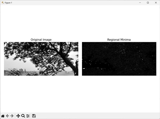
Using Custom Structuring Element

We can also use a custom structuring element to get the regional minima from an image.

In mahotas, while getting regional minima from an image we can use a custom structuring element to define how neighboring pixels are connected. We can use this to get a resultant image as per our need. It can by done by passing the structuring element to the Bc parameter in the regmin() function.

For example, let's consider the custom structuring element: [[1, 1, 1, 1, 0], [1, 1, 0, 1,1], [0, 1, 1, 1, 1], [1, 1, 1, 0, 1], [1, 0, 1, 1, 1]]. This structuring element implies horizontal and vertical connectivity. This means that only the pixels horizontally left or right and vertically above or below another pixel are considered its neighbors.

Example

Here, we are using a custom structuring element to get the regional minima of an image.

import mahotas as mh
import numpy as np
import matplotlib.pyplot as mtplt
# Loading the image
image = mh.imread('tree.tiff')
# Converting it to grayscale
image = mh.colors.rgb2gray(image)
# Setting custom structuring element
struct_element = np.array([[1, 1, 1, 1, 0],[1, 1, 0, 1, 1],
[0, 1, 1, 1, 1],[1, 1, 1, 0, 1],[1, 0, 1, 1, 1]])
# Getting the regional minima
regional_minima = mh.regmin(image, Bc=struct_element)
# Creating a figure and axes for subplots
fig, axes = mtplt.subplots(1, 2)
# Displaying the original image
axes[0].imshow(image, cmap='gray')
axes[0].set_title('Original Image')
axes[0].set_axis_off()
# Displaying the regional minima
axes[1].imshow(regional_minima, cmap='gray')
axes[1].set_title('Regional Minima')
axes[1].set_axis_off()
# Adjusting spacing between subplots
mtplt.tight_layout()
# Showing the figures
mtplt.show()

Output

Output of the above code is as follows −

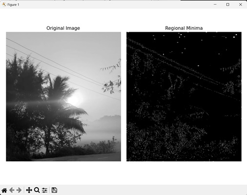
Using a Specific Region of an Image

We can also find the regional minima of a specific region of an image. A specific region of an image refers to a small part of a larger image. The specific region can be extracted by cropping the original image to remove unnecessary areas.

In mahotas, we can use a portion of an image and get its regional minima. First, we get the specific area from the original image by providing dimensions of the x and y axis.

Then we use the cropped image and get the regional minima using the regmin() function.

For example, let’s say we specify [:900, :800] as the dimensions of x and y axis respectively. Then, the specific region will be in range of 0 to 900 pixels for x−axis and 0 to 800 pixels for y−axis.

Example

In the example mentioned below, we are getting the regional minima within a specific region of an image.

import mahotas as mh
import numpy as np
import matplotlib.pyplot as mtplt
# Loading the image
image = mh.imread('sun.png')
# Converting it to grayscale
image = mh.colors.rgb2gray(image)
# Using specific regions of the image
image = image[:900, :800]
# Getting the regional minima
regional_minima = mh.regmin(image)
# Creating a figure and axes for subplots
fig, axes = mtplt.subplots(1, 2)
# Displaying the original image
axes[0].imshow(image, cmap='gray')
axes[0].set_title('Original Image')
axes[0].set_axis_off()
# Displaying the regional minima
axes[1].imshow(regional_minima, cmap='gray')
axes[1].set_title('Regional Minima')
axes[1].set_axis_off()
# Adjusting spacing between subplots
mtplt.tight_layout()
# Showing the figures
mtplt.show()

Output

After executing the above code, we get the following output −

Print Page