Mahotas - Histogram of Image

---

---

A histogram of an image refers to a graphical representation that shows the distribution of pixel intensities within the image. It provides information about the frequency of occurrence of different intensity values in the image.

The horizontal axis (X−aixs) of a histogram represents the range of possible intensity values in an image, while the vertical axis (Y−axis) represents the frequency or number of pixels that have a particular intensity value.

Histogram of Image in Mahotas

To compute the histogram of an image in Mahotas, we can use the fullhistogram() function provided by the library. This function will return an array representing the histogram values.

A histogram array contains bins representing possible pixel values in an image. Each bin corresponds to a specific intensity level, indicating the frequency or count of pixels with that particular value.

For example, in an 8−bit grayscale image, the histogram array has 256 bins representing intensity levels from 0 to 255.

The mahotas.fullhistogram() function

The mahotas.fullhistogram() function in Mahotas takes an image as input and returns an array representing the histogram. This function calculates the histogram by counting the number of pixels at each intensity level or bin.

Syntax

Following is the basic syntax of the fullhistogram() function in mahotas −

mahotas.fullhistogram(image)

Where, 'image' is the input image of an unsigned type.

Mahotas can handle only unsigned integer arrays in this function

Example

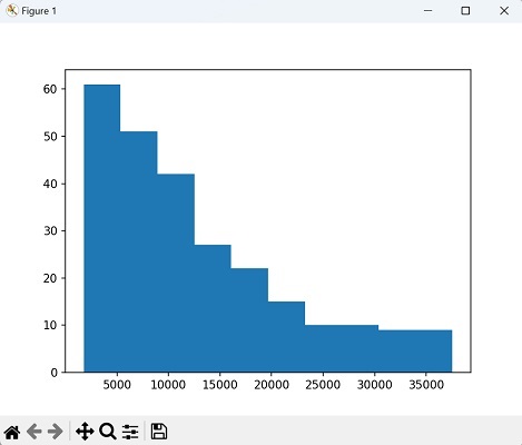
In the following example, we are trying to display the histogram of a colored image using the fullhistogram() function −

import mahotas as mh
import numpy as np
from pylab import imshow, show
import matplotlib.pyplot as plt
image = mh.imread('sun.png')
hist = mh.fullhistogram(image)
plt.hist(hist)
plt.show()

Output

After executing the above code, we get the following output −

Grayscale Image Histogram

The grayscale image histogram in mahotas refers to a representation of the distribution of pixel intensities in a grayscale image.

The grayscale images generally have pixel intensities ranging from 0 (black) to 255 (white). By default, Mahotas considers the full range of pixel intensities when calculating the histogram.

This means that all intensities from 0 to 255 are included in the histogram calculation.

By considering 256 bins and the full range of pixel intensities, Mahotas provides a comprehensive representation of the distribution of pixel intensities in the grayscale image.

Example

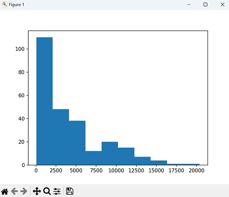
In here, we are trying to display the grayscale image histogram using mahotas −

import mahotas as mh
import numpy as np
import matplotlib.pyplot as plt
# Convert image array to uint8 type
image = mh.imread('sun.png', as_grey=True).astype(np.uint8)
hist = mh.fullhistogram(image)
plt.hist(hist)
plt.show()

Output

The output produced is as shown below −

Blue Channel RGB Image Histogram

The blue channel contains the information about the blue color component of each pixel.

We will use the mahotas library in conjunction with numpy and matplotlib to extract the blue channel from an RGB image.

We can extract the blue channel from the RGB image by selecting the third (index 2) channel using array slicing. This gives us a grayscale image representing the blue component intensities.

Then, using numpy, we calculate the histogram of the blue channel. We flatten the blue channel array to create a 1D array, ensuring that the histogram is computed over all the pixels in the image.

Finally, we use matplotlib to visualize the histogram.

Example

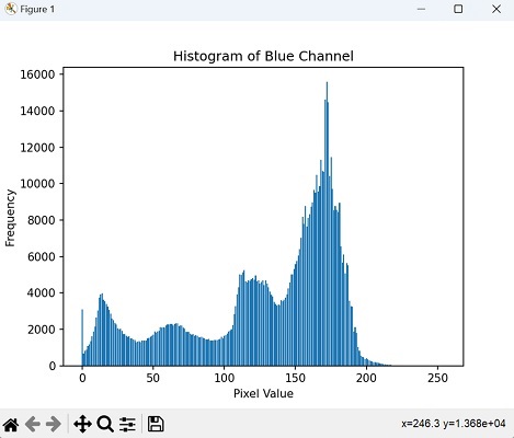
Now, we are trying to display the RGB image histogram of blue channel −

import mahotas as mh
import numpy as np
import matplotlib.pyplot as plt
# Loading RGB image
image = mh.imread('sea.bmp')
# Extracting the blue channel
blue_channel = image[:, :, 2]
# Calculating the histogram using numpy
hist, bins = np.histogram(blue_channel.flatten(), bins=256, range=[0, 256])
# Plot histogram
plt.bar(range(len(hist)), hist)
plt.xlabel('Pixel Value')
plt.ylabel('Frequency')
plt.title('Histogram of Blue Channel')
plt.show()

Output

Following is the output of the above code −