Mahotas - Distance Transform

Distance transformation is a technique that calculates the distance between each pixel and the nearest background pixel. Distance transformation works on distance metrics, which define how the distance between two points is calculated in a space.

Applying distance transformation on an image creates the distance map. In the distance map, dark shades are assigned to the pixels near the boundary, indicating a short distance, and lighter shades are assigned to pixels further away, indicating a larger distance to the nearest background pixel.

Distance Transform in Mahotas

In Mahotas, we can use the mahotas.distance() function to perform distance transformation on an image. It uses an iterative approach to create a distance map.

The function first initializes the distance values for all pixels in the image. The background pixels are assigned a distance value of infinity, while the foreground pixels are assigned a distance value of zero.

Then, the function updates the distance value of each background pixel based on the distances of its neighboring pixels. This occurs until all the distance value of all the background pixels has been computed.

The mahotas.distance() function

The mahotas.distance() function takes an image as input and returns a distance map as output. The distance map is an image that contains the distance between each pixel in the input image and the nearest background pixel.

Syntax

Following is the basic syntax of the distance() function in mahotas −

mahotas.distance(bw, metric='euclidean2')

Where,

bw − It is the input image.
metric (optional) − It specifies the type of distance used to determine the distance between a pixel and a background pixel (default is euclidean2).

Example

In the following example, we are performing distance transformation on an image using the mh.distance() function.

import mahotas as mh
import numpy as np
import matplotlib.pyplot as mtplt
# Loading the image
image = mh.imread('nature.jpeg')
# Converting it to grayscale
image = mh.colors.rgb2gray(image)
# Finding distance map
distance_map = mh.distance(image)
# Creating a figure and axes for subplots
fig, axes = mtplt.subplots(1, 2)
# Displaying the original image
axes[0].imshow(image)
axes[0].set_title('Original Image')
axes[0].set_axis_off()
# Displaying the distance transformed image
axes[1].imshow(distance_map)
axes[1].set_title('Distance Transformed Image')
axes[1].set_axis_off()
# Adjusting spacing between subplots
mtplt.tight_layout()
# Showing the figures
mtplt.show()

Output

Following is the output of the above code −

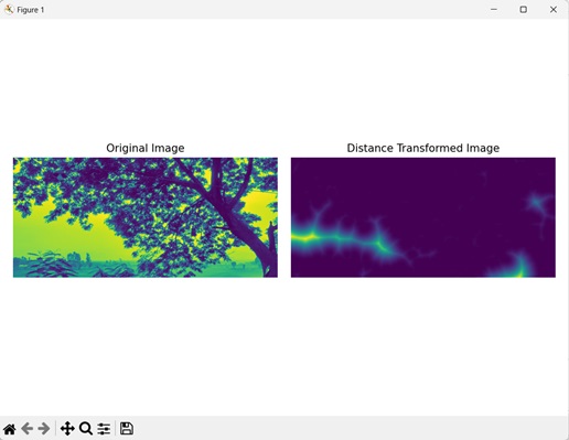
Using Labeled Image

We can also perform distance transformation using a labeled image. A labeled image refers to an image where distinct regions are assigned unique labels for segmenting the image into different regions.

In mahotas, we can apply distance transformation on an input image by first reducing its noise using the mh.gaussian_filter() function. Then, we use the mh.label() function to separate the foreground regions from the background regions.

We can then create a distance map using the mh.distance() function. This will calculate the distance between the pixels of the foreground regions and the pixels of the background region.

Example

In the example mentioned below, we are finding the distance map of a filtered labeled image.

import mahotas as mh
import numpy as np
import matplotlib.pyplot as mtplt
# Loading the image
image = mh.imread('tree.tiff')
# Converting it to grayscale
image = mh.colors.rgb2gray(image)
# Applying gaussian filtering
gauss_image = mh.gaussian_filter(image, 3)
gauss_image = (gauss_image > gauss_image.mean())
# Converting it to a labeled image
labeled, num_objects = mh.label(gauss_image)
# Finding distance map
distance_map = mh.distance(labeled)
# Creating a figure and axes for subplots
fig, axes = mtplt.subplots(1, 2)
# Displaying the original image
axes[0].imshow(image)
axes[0].set_title('Original Image')
axes[0].set_axis_off()
# Displaying the distance transformed image
axes[1].imshow(distance_map)
axes[1].set_title('Distance Transformed Image')
axes[1].set_axis_off()
# Adjusting spacing between subplots
mtplt.tight_layout()
# Showing the figures
mtplt.show()

Output

Output of the above code is as follows

Using Euclidean Distance

Another way of performing distance transformation on an image is using euclidean distance. Euclidean distance is the straight-line distance between two points in a coordinate system. It is calculated as the square root of the sum of squared differences between the coordinates.

For example, let's say there are two points A and B with coordinate values of (2, 3) and (5, 7) respectively. Then the squared difference of x and y coordinate will be (5−2)² = 9 and (7−3)² = 16. Sum of the square will be 9 + 16 = 25 and square root of this will be 5, which is the euclidean distance between point A and point B.

In mahotas, we can use euclidean distance instead of the default euclidean2 as the distance metric. To do this, we pass the value 'euclidean' to the metric parameter.

Note − The euclidean should be written as 'euclidean' (in single quotes), since the data type of metric parameter is string.

Example

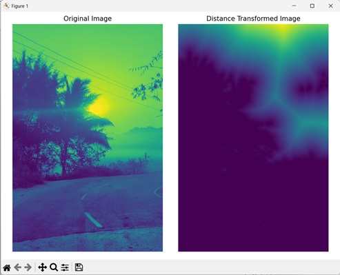
In this example, we are using euclidean distance type for distance transformation of an image.

import mahotas as mh
import numpy as np
import matplotlib.pyplot as mtplt
# Loading the image
image = mh.imread('sun.png')
# Converting it to grayscale
image = mh.colors.rgb2gray(image)
# Applying gaussian filtering
gauss_image = mh.gaussian_filter(image, 3)
gauss_image = (gauss_image > gauss_image.mean())
# Finding distance map
distance_map = mh.distance(gauss_image, metric='euclidean')
# Creating a figure and axes for subplots
fig, axes = mtplt.subplots(1, 2)
# Displaying the original image
axes[0].imshow(image)
axes[0].set_title('Original Image')
axes[0].set_axis_off()
# Displaying the distance transformed image
axes[1].imshow(distance_map)
axes[1].set_title('Distance Transformed Image')
axes[1].set_axis_off()
# Adjusting spacing between subplots
mtplt.tight_layout()
# Showing the figures
mtplt.show()

Output

After executing the above code, we get the following output −

Print Page