Mahotas - Filtering Regions

---

---

Filtering regions refers to excluding specific regions of a labeled image based on certain criteria. A commonly used criteria for filtering regions is based on their size. By specifying a size limit, regions that are either too small or too large can be excluded to get a clean output image.

Another criterion for filtering regions is to check whether a region is bordered or not. By applying these filters, we can selectively remove or retain regions of interest in the image.

Filtering Regions in Mahotas

In Mahotas, we can convert filter regions of a labeled image by using the labeled.filter_labeled() function. This function applies filters to the selected regions of an image while leaving other regions unchanged.

Using the mahotas.labeled.filter_labeled() Function

The mahotas.labeled.filter_labeled() function takes a labeled image as input and removes unwanted regions based on certain properties. It identifies the regions based on the labels of an image.

The resultant image consists of only regions that match the filter criterion.

Syntax

Following is the basic syntax of the filter_labeled() function in mahotas −

mahotas.labeled.filter_labeled(labeled, remove_bordering=False, min_size=None,
max_size=None)

where,

• labeled − It is the array.

• remove_bordering (optional) − It defines whether to remove regions touching the border.

• min_size (optional) − It is the minimum size of the region that needs to be kept (default is no minimum).

• max_size (optional) − It is the maximum size of the region that needs to be kept (default is no maximum).

Example

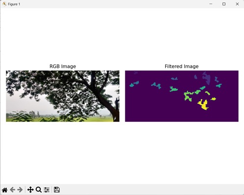
In the following example, we are filtering a labeled image to remove border pixels.

import mahotas as mh
import numpy as np
import matplotlib.pyplot as mtplt
# Loading the image
image_rgb = mh.imread('tree.tiff')
image = image_rgb[:,:,0]
# Applying gaussian filtering
image = mh.gaussian_filter(image, 4)
image = (image > image.mean())
# Converting it to a labeled image
labeled, num_objects = mh.label(image)
# Applying filters
filtered_image, num_objects = mh.labeled.filter_labeled(labeled,
remove_bordering=True)
# Creating a figure and axes for subplots
fig, axes = mtplt.subplots(1, 2)
# Displaying the original RGB image
axes[0].imshow(image_rgb)
axes[0].set_title('RGB Image')
axes[0].set_axis_off()
# Displaying the filtered image
axes[1].imshow(filtered_image)
axes[1].set_title('Filtered Image')
axes[1].set_axis_off()
# Adjusting spacing between subplots
mtplt.tight_layout()
# Showing the figures
mtplt.show()

Output

Following is the output of the above code −

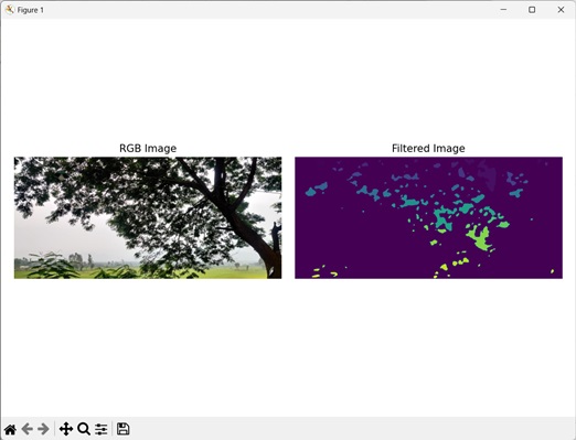
Filtering on Regions of Specific Size

We can also filter regions of specific size in an image. In this way, we can remove regions from labeled images which do not fall within a specific size limit (regions that are too small or too large).

In mahatos, we can achieve this by specifying values to the optional parameter min_size and max_size in the labeled.filter_label() function.

Example

The following example shows filtering a labeled image to remove regions of specific size.

import mahotas as mh
import numpy as np
import matplotlib.pyplot as mtplt
# Loading the image
image_rgb = mh.imread('tree.tiff')
image = image_rgb[:,:,0]
# Applying gaussian filtering
image = mh.gaussian_filter(image, 4)
image = (image > image.mean())
# Converting to a labeled image
labeled, num_objects = mh.label(image)
# Applying filters
filtered_image, num_objects = mh.labeled.filter_labeled(labeled, min_size=10,
max_size=50000)
# Create a figure and axes for subplots
fig, axes = mtplt.subplots(1, 2)
# Displaying the original RGB image
axes[0].imshow(image_rgb)
axes[0].set_title('RGB Image')
axes[0].set_axis_off()
# Displaying the filtered image
axes[1].imshow(filtered_image)
axes[1].set_title('Filtered Image')
axes[1].set_axis_off()
# Adjusting spacing between subplots
mtplt.tight_layout()
# Showing the figures
mtplt.show()

Output

Output of the above code is as follows −

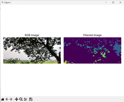
Filtering on Border Regions and Regions of Specific Size

We can filter bordered regions along with regions of a specific size in an image. In this, we remove regions which touch the border and regions which do not fall within a specific size limit.

In mahotas, we can do this by specifying values to the optional parameter min_size and max_size and setting the optional parameter remove_bordering to True in the labeled.filter_label() function.

Example

In this example, a filter is applied to remove border regions and regions of specific size of a labeled image.

import mahotas as mh
import numpy as np
import matplotlib.pyplot as mtplt
# Loading the image
image_rgb = mh.imread('tree.tiff')
image = image_rgb[:,:,0]
# Applying gaussian filtering
image = mh.gaussian_filter(image, 4)
image = (image > image.mean())
# Converting it to a labeled image
labeled, num_objects = mh.label(image)
# Applying filters
filtered_image, num_objects = mh.labeled.filter_labeled(labeled,
remove_bordering=True, min_size=1000, max_size=50000)
# Creating a figure and axes for subplots
fig, axes = mtplt.subplots(1, 2)
# Displaying the original RGB image
axes[0].imshow(image_rgb)
axes[0].set_title('RGB Image')
axes[0].set_axis_off()
# Displaying the filtered image
axes[1].imshow(filtered_image)
axes[1].set_title('Filtered Image')
axes[1].set_axis_off()
# Adjusting spacing between subplots
mtplt.tight_layout()
# Showing the figures
mtplt.show()

Output

The output produced is as shown below −