Mahotas - Morphological Operators

Morphological operators are a set of image processing techniques that help modify the shape, size, and spatial relationships of objects in an image. They are like tools used to reshape or manipulate the objects within an image.

Imagine you have a picture with various objects like circles, squares, and lines. Morphological operators allow you to change the appearance of these objects in different ways.

For example, you can make them bigger or smaller, smooth their edges, remove tiny details, or fill in gaps.

To achieve these transformations, morphological operators use mathematical operations that involve scanning the image with a special pattern called a structuring element. This structuring element defines the shape and size of the neighborhood around each pixel that will be considered during the operation.

Mahotas and Morphological Operators

Mahotas provides a comprehensive set of morphological operators that can be applied to binary, grayscale, or multichannel images. These operators are implemented efficiently using optimized algorithms, making them suitable for real−world applications with largescale datasets.

Let us look at few morphological operations which can be done in mahotas −

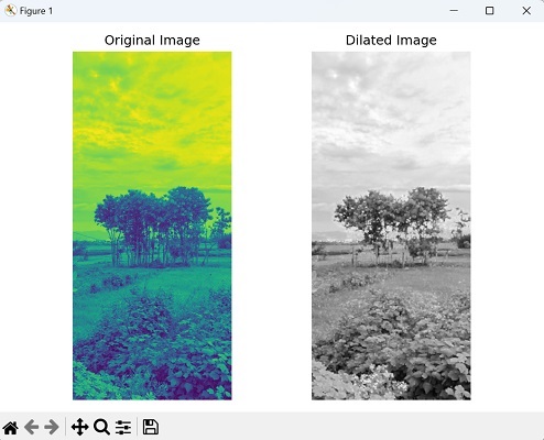
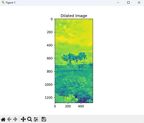
Dilation

Dilation is a morphological operation that expands the pixels on the boundaries of objects in an image. It involves scanning the image with a structuring element and replacing each pixel with the maximum value within the corresponding neighborhood defined by the structuring element.

Let us look at the dilated image along with the original image below −

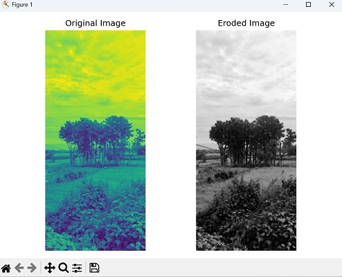
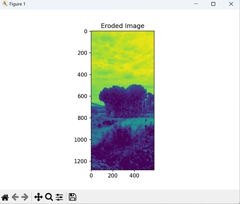
Erosion

Erosion is a basic morphological operator that shrinks or erodes the pixels on boundaries of objects in an image.

Following is the eroded image along with its original image −

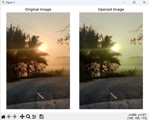
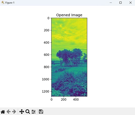
Opening

Opening is a combination of erosion followed by dilation. It removes small objects and fills in small holes in the foreground while preserving the overall shape and connectivity of larger objects.

Let us look at the opened image in mahotas −

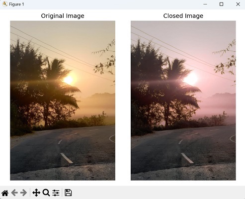
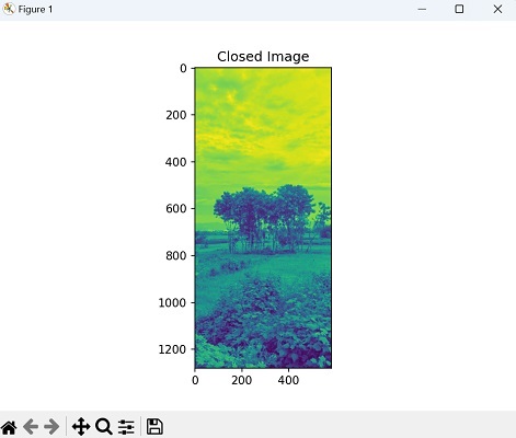
Closing

Closing is the reverse of opening, consisting of dilation followed by erosion. It fills small gaps and holes within the foreground, ensuring the connectivity of objects.

Now, let us look at the closed image in mahotas −

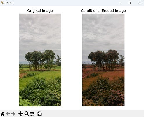
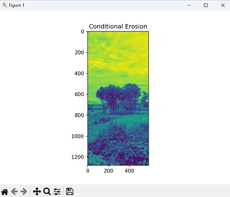
Conditional Erosion

Conditional erosion is a morphological operation that preserves structures in an image based on a user−defined condition. It selectively erodes regions of an image based on the condition specified by a second image called the marker image.

The operation erodes the image only where the marker image has non−zero values.

Following image shows conditional erosion −

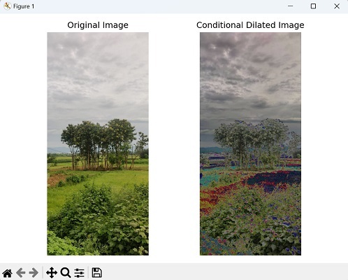
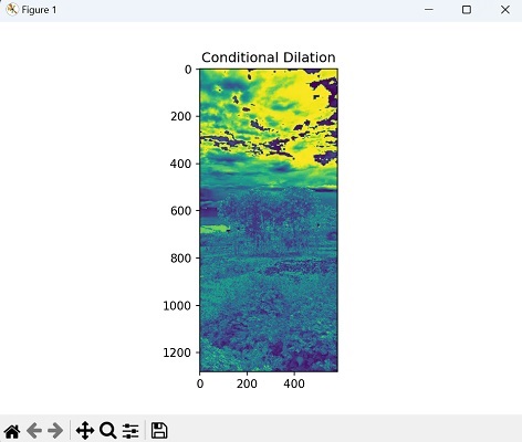
Conditional Dilation

Conditional dilation is similar to conditional erosion but operates in the opposite way. It selectively dilates regions of an image based on the condition specified by the marker image.

The operation dilates the image only where the marker image has non−zero values.

Following image shows conditional dilation −

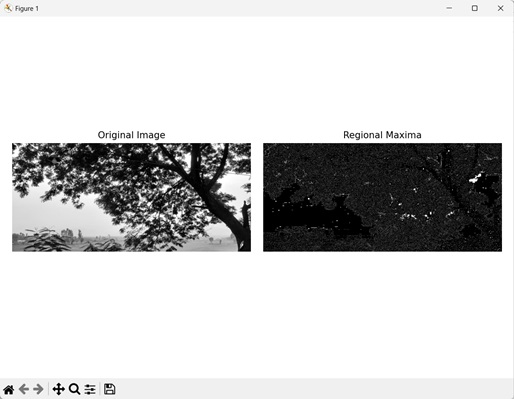
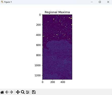
Regional Maxima

Regional maxima are points in an image that have the highest intensity within their neighborhood. They represent local peaks or salient features in the image.

The regional maxima operator in Mahotas identifies these local maxima and marks them as foreground pixels.

Following image represents regional maxima −

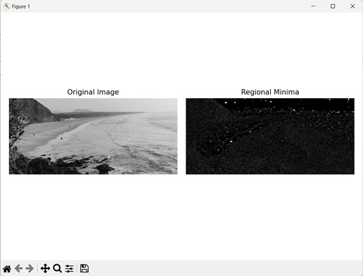
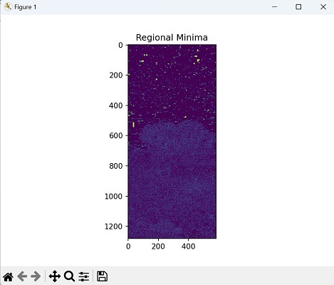
Regional Minima

Regional minima are points in an image that have the lowest intensity within their neighborhood. They represent local basins or depressions in the image.

The regional minima operator in Mahotas identifies these local minima and marks them as background pixels.

Following image represents regional minima −

Example

In the following example, we are trying to perform all the above explained morphological operations −

import mahotas as mh
import matplotlib.pyplot as plt
import numpy as np
image = mh.imread('nature.jpeg', as_grey=True).astype(np.uint8)
# Dilation
dilated_image = mh.dilate(image, Bc=mh.disk(8))
plt.title("Dilated Image")
plt.imshow(dilated_image)
plt.show()
# Erosion
plt.title("Eroded Image")
eroded_image = mh.erode(image, Bc=mh.disk(8))
plt.imshow(eroded_image)
plt.show()
# Opening
plt.title("Opened Image")
opened_image = mh.open(image)
plt.imshow(opened_image)
plt.show()
# Closing
plt.title("Closed Image")
closed_image = mh.close(image)
plt.imshow(closed_image)
plt.show()
# Conditional Dilation
plt.title("Conditional Dilation")
g = image * 6
cdilated_image = mh.cdilate(image, g)
plt.imshow(cdilated_image)
plt.show()
# Conditional Erosion
plt.title("Conditional Erosion")
scaled_image = image * 0.5
scaled_image = scaled_image.astype(np.uint8)
ceroded_image = mh.cerode(image, scaled_image)
plt.imshow(ceroded_image)
plt.show()
# Regional Maxima
plt.title("Regional Maxima")
regional_maxima = mh.regmax(image)
plt.imshow(regional_maxima)
plt.show()
# Regional Minima
plt.title("Regional Minima")
regional_minima = mh.regmin(image)
plt.imshow(regional_minima)
plt.show()