Mahotas - Convolution of Image

Convolution in image processing is used to perform various filter operations on an image.

Here are some of them −

Extract features − It is used to detect the features such as edges, corners, blobs, etc. by applying specific filters.
Filtering − It is used to perform smoothing and sharpening operationson an image.
Compression − we can compress the image by removing the redundant information in the image.

Convolution of an Image in Mahotas

In Mahotas, you can perform convolution on an image using the convolve() function. This function takes two arguments− the input image and the kernel; where, the kernel is a small matrix that defines the operation to be applied during convolution, such as blurring, sharpening, edge detection, or any other desired effect.

Using the convolve() Function

The convolve() function is used to perform convolution on an image. Convolution is a mathematical operation that takes two arrays− image and convolution kernel, and produces a third array (output image).

The convolution kernel is a small array of numbers that is used to filter the image. The convolution operation is performed by multiplying the corresponding elements of the image and the kernel, and then adding the results together. The output of the convolution operation is a new image that has been filtered by the kernel.

Following syntax to perform convolution in mahotas −

convolve(image, kernel, mode='reflect', cval=0.0, out=None)

where,

image − It is the input image.
kernel − It is the convolution kernel.
mode − It specifies how to handle the edges of the image. It can be reflect, nearest constant, ignore, wrap, or mirror. Reflect is selected as default.
cval − It specifies the value to use for pixels that are outside of the image.
out − It specifies the output image. If the out argument is not specified, a new image will be created.

Example

In the following example, we first resize the input image 'nature.jpeg' to a '4×4' shape using mh.imresize() function. Then, we create a '4×4' kernel with all values set to 1. Finally, we use the mh.convolve() function to perform convolution −

import mahotas as mh
import numpy as np
# Load the image
image = mh.imread('nature.jpeg', as_grey=True)
# Resize the image to 4x4
image = mh.imresize(image, (4, 4))
# Create a 4x4 kernel
kernel = np.ones((4, 4))
# Perform convolution
result = mh.convolve(image, kernel)
print (result)

Output

Following is the output of the above code −

[[3155.28 3152.84 2383.42 1614. ]
[2695.96 2783.18 2088.38 1393.58]
[1888.48 1970.62 1469.53 968.44]
[1081. 1158.06 850.68 543.3 ]]

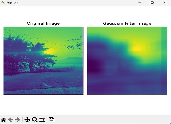
Convolution with a Gaussian Kernel

A Gaussian kernel in Mahotas is a small matrix of numbers that is used to blur or smoothen an image.

The Gaussian kernel applies a weighted average to each pixel, where the weights are determined by a bell−shaped curve called the Gaussian distribution. The kernel gives higher weights to nearby pixels and lower weights to distant ones. This process helps to reduce noise and enhance features in the image, resulting in a smoother and more visually pleasing output.

Following is the basic syntax of Gaussian kernel in mahotas −

mahotas.gaussian_filter(array, sigma)

Where,

array − It is the input array.
sigma − It is the standard deviation for Gaussian kernel.

Example

Following is an example of convolving an image with gaussian filter. Here, we are resizing the image, converting it to grayscale, applying a Gaussian filter to blur the image, and then displaying the original and blurred images side by side −

import mahotas as mh
import matplotlib.pyplot as mtplt
# Load the image
image = mh.imread('sun.png')
# Convert to grayscale if needed
if len(image.shape) > 2:
   image = mh.colors.rgb2gray(image)
# Resize the image to 128x128
image = mh.imresize(image, (128, 128))
# Create the Gaussian kernel
kernel = mh.gaussian_filter(image, 1.0)
# Reduce the size of the kernel to 20x20
kernel = kernel[:20, :20]
# Blur the image
blurred_image = mh.convolve(image, kernel)
# Creating a figure and subplots
fig, axes = mtplt.subplots(1, 2)
# Displaying original image
axes[0].imshow(image)
axes[0].axis('off')
axes[0].set_title('Original Image')
# Displaying blurred image
axes[1].imshow(blurred_image)
axes[1].axis('off')
axes[1].set_title('Gaussian Filter Image')
# Adjusting the spacing and layout
mtplt.tight_layout()
# Showing the figure
mtplt.show()

Output

Output of the above code is as follows −

Convolution with Padding

Convolution with padding in Mahotas resfers to adding extra pixels or border around the edges of an image. before performing the convolution operation. The purpose of padding is to create a new image with increased dimensions, without losing information from the original image's edges.

Padding ensures that the kernel can be applied to all pixels, including those at the edges, resulting in a convolution output with the same size as the original image.

Example

Here, we have defined a custom kernel as a NumPy array to emphasize the edges of the image −

import numpy as np
import mahotas as mh
import matplotlib.pyplot as mtplt
# Create a custom kernel
kernel = np.array([[0, -1, 0],[-1, 5, -1],
[0, -1, 0]])
# Load the image
image = mh.imread('sea.bmp', as_grey=True)
# Add padding to the image
padding = np.pad(image, 150, mode='wrap')
# Perform convolution with padding
padded_image = mh.convolve(padding, kernel)
# Creating a figure and subplots
fig, axes = mtplt.subplots(1, 2)
# Displaying original image
axes[0].imshow(image)
axes[0].axis('off')
axes[0].set_title('Original Image')
# Displaying padded image
axes[1].imshow(padded_image)
axes[1].axis('off')
axes[1].set_title('Padded Image')
# Adjusting the spacing and layout
mtplt.tight_layout()
# Showing the figure
mtplt.show()

Output

After executing the above code, we get the following output −

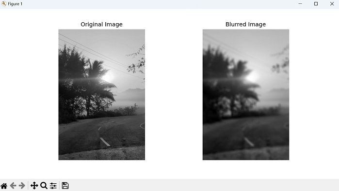
Convolution with a Box Filter for Blurring

Convolution with a box filter in Mahotas is a technique that can be used for blurring images. A box filter is a simple filter where each element in the filter kernel has the same value, resulting in a uniform weight distribution.

Convolution with a box filter involves sliding the kernel over the image and taking the average of the pixel values in the region covered by the kernel. This average value is then used to replace the center pixel value in the output image.

The process is repeated for all pixels in the image, resulting in a blurred version of the original image. The amount of blurring is determined by the size of the kernel, with larger kernels resulting in more blur.

Example

Following is an example of performing convolution with a box filter to blur the image −

import mahotas as mh
import numpy as np
import matplotlib.pyplot as plt
# Load the image
image = mh.imread('sun.png', as_grey=True)
# Define the size of the box filter
box_size = 25
# Create the box filter
box_filter = np.ones((box_size, box_size)) / (box_size * box_size)
# Perform convolution with the box filter
blurred_image = mh.convolve(image, box_filter)
# Display the original and blurred images
fig, axes = plt.subplots(1, 2, figsize=(10, 5))
axes[0].imshow(image, cmap='gray')
axes[0].set_title('Original Image')
axes[0].axis('off')
axes[1].imshow(blurred_image, cmap='gray')
axes[1].set_title('Blurred Image')
axes[1].axis('off')
plt.show()

Output

We get the output as shown below −

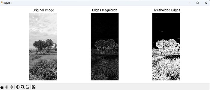
Convolution with a Sobel Filter for Edge Detection

A Sobel filter is commonly used for edge detection. It consists of two separate filters− one for detecting horizontal edges and another for vertical edges.

By convolving the Sobel filter with an image, we obtain a new image where the edges are highlighted and the rest of the image appears blurred. The highlighted edges typically have higher intensity values compared to the surrounding areas.

Example

In here, we are performing edge detection using Sobel filters by convolving them with a grayscale image. We are then computing the magnitude of the edges and applying a threshold to obtain a binary image of the detected edges −

import mahotas as mh
import numpy as np
import matplotlib.pyplot as plt
image = mh.imread('nature.jpeg', as_grey=True)
# Apply Sobel filter for horizontal edges
sobel_horizontal = np.array([[1, 2, 1],
[0, 0, 0],[-1, -2, -1]])
# convolving the image with the filter kernels
edges_horizontal = mh.convolve(image, sobel_horizontal)
# Apply Sobel filter for vertical edges
sobel_vertical = np.array([[1, 0, -1],[2, 0, -2],[1, 0, -1]])
# convolving the image with the filter kernels
edges_vertical = mh.convolve(image, sobel_vertical)
# Compute the magnitude of the edges
edges_magnitude = np.sqrt(edges_horizontal**2 + edges_vertical**2)
# Threshold the edges
threshold = 50
thresholded_edges = edges_magnitude > threshold
# Display the original image and the detected edges
fig, axes = plt.subplots(1, 3, figsize=(12, 4))
axes[0].imshow(image, cmap='gray')
axes[0].set_title('Original Image')
axes[0].axis('off')
axes[1].imshow(edges_magnitude, cmap='gray')
axes[1].set_title('Edges Magnitude')
axes[1].axis('off')
axes[2].imshow(thresholded_edges, cmap='gray')
axes[2].set_title('Thresholded Edges')
axes[2].axis('off')
plt.tight_layout()
plt.show()

Output

The output obtained is as follows −

Print Page