Mahotas - Labeling Images

Labeling images refers to assigning categories (labels) to different regions of an image. The labels are generally represented as integer values, where each value corresponds to a specific category or region.

For example, let's consider an image with various objects or regions. Each region is assigned a unique value (integer) to differentiate it from other regions. The background region is labeled with a value of 0.

Labeling Images in Mahotas

In Mahotas, we can label images using label() or labeled.label() functions.

These functions segment an image into distinct regions by assigning unique labels or identifiers to different connected components within an image. Each connected component is a group of adjacent pixels that share a common property, such as intensity or color.

The labeling process creates an image where pixels belonging to the same region are assigned the same label value.

Using the mahotas.label() Function

The mahotas.label() function takes an image as input, where regions of interest are represented by foreground (non−zero) values and the background is represented by zero.

The function returns the labeled array, where each connected component or region is assigned a unique integer label.

The label() function performs labeling using 8−connectivity, which refers to the relationship between pixels in an image, where each pixel is connected to its eight surrounding neighbors, including the diagonals.

Syntax

Following is the basic syntax of the label() function in mahotas −

mahotas.label(array, Bc={3x3 cross}, output={new array})

where,

array − It is the input array.
Bc (optional) − It is the structuring element used for connectivity.
output (optional) − It is the output array (defaults to new array of same shape as array).

Example

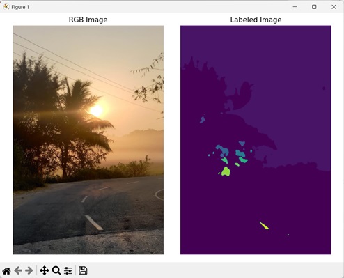
In the following example, we are labeling an image using the mh.label() function.

import mahotas as mh
import numpy as np
import matplotlib.pyplot as mtplt
# Loading the image
image_rgb = mh.imread('sun.png')
image = image_rgb[:,:,0]
# Applying gaussian filtering
image = mh.gaussian_filter(image, 4)
image = (image > image.mean())
# Converting it to a labeled image
labeled, num_objects = mh.label(image)
# Creating a figure and axes for subplots
fig, axes = mtplt.subplots(1, 2)
# Displaying the original RGB image
axes[0].imshow(image_rgb)
axes[0].set_title('RGB Image')
axes[0].set_axis_off()
# Displaying the labeled image
axes[1].imshow(labeled)
axes[1].set_title('Labeled Image')
axes[1].set_axis_off()
# Adjusting spacing between subplots
mtplt.tight_layout()
# Showing the figures
mtplt.show()

Output

Following is the output of the above code −

Using the mahotas.labeled.label() Function

The mahotas.labeled.label() function assigns consecutive labels starting from 1 to different regions of an image. It works similar to mahotas.label() function to segment an image into distinct regions.

If you have a labeled image with non−sequential label values, the labeled.label() function updates the label values to be in sequential order.

For example, let’s say we have a labeled image with four regions having labels 2, 4, 7, and 9. The labeled.label() function will transform the image into a new labeled image with consecutive labels 1, 2, 3, and 4 respectively.

Syntax

Following is the basic syntax of the labeled.label() function in mahotas −

mahotas.labeled.label(array, Bc={3x3 cross}, output={new array})

where,

array − It is the input array.
Bc (optional) − It is the structuring element used for connectivity.
output (optional) − It is the output array (defaults to new array of same shape as array).

Example

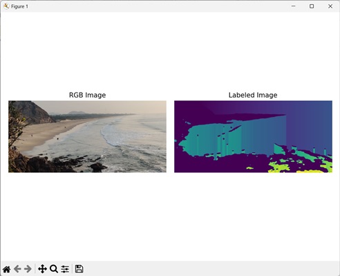
The following example shows conversion of an image to a labeled image using mh.labeled.label() function.

import mahotas as mh
import numpy as np
import matplotlib.pyplot as mtplt
# Loading the image
image_rgb = mh.imread('sea.bmp')
image = image_rgb[:,:,0]
# Applying gaussian filtering
image = mh.gaussian_filter(image, 4)
image = (image > image.mean())
# Converting it to a labeled image
labeled, num_objects = mh.labeled.label(image)
# Creating a figure and axes for subplots
fig, axes = mtplt.subplots(1, 2)
# Displaying the original RGB image
axes[0].imshow(image_rgb)
axes[0].set_title('RGB Image')
axes[0].set_axis_off()
# Displaying the labeled image
axes[1].imshow(labeled)
axes[1].set_title('Labeled Image')
axes[1].set_axis_off()
# Adjusting spacing between subplots
mtplt.tight_layout()
# Showing the figures
mtplt.show()

Output

Following is the output of the above code −

Using Custom Structuring Element

We can use a custom structuring element with the label functions to segment an image as per the requirement. A structuring element is a binary array of odd dimensions consisting of ones and zeroes that defines the connectivity pattern of the neighborhood pixels during image labeling.

The ones indicate the neighboring pixels that are included in the connectivity analysis, while the zeros represent the neighbors that are excluded or ignored.

For example, let's consider the custom structuring element: [[1, 0, 0], [0, 1, 0], [0, 0,1]]. This structuring element implies diagonal connectivity. It means that for each pixel in the image, only the pixels diagonally above and below it is considered its neighbors during the labeling or segmentation process.

Example

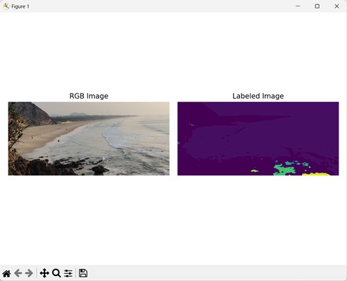
Here, we have defined a custom structuring element to label an image.

import mahotas as mh
import numpy as np
import matplotlib.pyplot as mtplt
# Loading the image
image_rgb = mh.imread('sea.bmp')
image = image_rgb[:,:,0]
# Applying gaussian filtering
image = mh.gaussian_filter(image, 4)
image = (image > image.mean())
# Creating a custom structuring element
binary_closure = np.array([[0, 1, 0],
[0, 1, 0],
[0, 1, 0]])
# Converting it to a labeled image
labeled, num_objects = mh.labeled.label(image, Bc=binary_closure)
# Creating a figure and axes for subplots
fig, axes = mtplt.subplots(1, 2)
# Displaying the original RGB image
axes[0].imshow(image_rgb)
axes[0].set_title('RGB Image')
axes[0].set_axis_off()
# Displaying the labeled image
axes[1].imshow(labeled)
axes[1].set_title('Labeled Image')
axes[1].set_axis_off()
# Adjusting spacing between subplots
mtplt.tight_layout()
# Showing the figure
mtplt.show()

Output

After executing the above code, we get the following output −

Print Page