Mahotas - Bernsen Local Thresholding

Bernsen local thresholding is a technique used for segmenting images into foreground and background regions. It uses intensity variations in a local neighborhood to assign a threshold value to each pixel in an image.

The size of the local neighborhood is determined using a window. A large window size considers more neighboring pixels in the thresholding process, creating smoother transitions between regions but removing finer details.

On the other hand, a small window size captures more details but may be susceptible to noise.

The difference between Bernsen local thresholding and other thresholding techniques is that Bernsen local thresholding uses a dynamic threshold value, while the other thresholding techniques use a single threshold value to separate foreground and background regions.

Bernsen Local Thresholding in Mahotas

In Mahotas, we can use the thresholding.bernsen() and thresholding.gbernsen() functions to apply Bernsen local thresholding on an image. These functions create a window of a fixed size and calculate the local contrast range of each pixel within the window to segment the image.

The local contrast range is the minimum and maximum grayscale values within the window.

The threshold value is then calculated as the average of minimum and maximum grayscale values. If the pixel intensity is higher than the threshold, it is assigned to the foreground (white), otherwise it is assigned to the background (black).

The window is then moved across the image to cover all the pixels to create a binary image, where the foreground and background regions are separated based on local intensity variations.

The mahotas.tresholding.bernsen() function

The mahotas.thresholding.bernsen() function takes a grayscale image as input and applies Bernsen local thresholding on it. It outputs an image where each pixel is assigned a value of 0 (black) or 255 (white).

The foreground pixels correspond to the regions of the image that have a relatively high intensity, whereas the background pixels correspond to the regions of the image that have a relatively low intensity.

Syntax

Following is the basic syntax of the bernsen() function in mahotas −

mahotas.thresholding.bernsen(f, radius, contrast_threshold, gthresh={128})

where,

f − It is the input grayscale image.
radius − It is the size of the window around each pixel.
contrast_threshold − It is the local threshold value.
gthresh (optional) − It is the global threshold value (default is 128).

Example

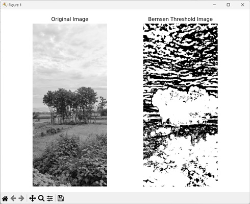
The following example shows the usage of mh.thresholding.bernsen() function to apply Bernsen local thresholding on an image.

import mahotas as mh
import numpy as np
import matplotlib.pyplot as mtplt
# Loading the image
image = mh.imread('nature.jpeg')
# Converting it to grayscale
image = mh.colors.rgb2gray(image)
# Creating Bernsen threshold image
threshold_image = mh.thresholding.bernsen(image, 5, 200)
# Creating a figure and axes for subplots
fig, axes = mtplt.subplots(1, 2)
# Displaying the original image
axes[0].imshow(image, cmap='gray')
axes[0].set_title('Original Image')
axes[0].set_axis_off()
# Displaying the threshold image
axes[1].imshow(threshold_image, cmap='gray')
axes[1].set_title('Bernsen Threshold Image')
axes[1].set_axis_off()
# Adjusting spacing between subplots
mtplt.tight_layout()
# Showing the figures
mtplt.show()

Output

Following is the output of the above code −

The mahotas.thresholding.gbernsen() function

The mahotas.thresholding.gbernsen() function also applies Bernsen local thresholding on an input grayscale image.

It is the generalized version of Bernsen local thresholding algorithm. It outputs a segmented image where each pixel is assigned a value of 0 or 255 depending on whether it is background or foreground.

The difference between gbernsen() and bernsen() function is that the gbernsen() function uses a structuring element to define the local neighborhood, while the bernsen() function uses a window of fixed size to define the local neighborhood around a pixel.

Also, gbernsen() calculates the threshold value based on the contrast threshold and the global threshold, while bernsen() only uses the contrast threshold to calculate the threshold value of each pixel.

Syntax

Following is the basic syntax of the gbernsen() function in mahotas −

mahotas.thresholding.gbernsen(f, se, contrast_threshold, gthresh)

Where,

f − It is the input grayscale image.
se − It is the structuring element.
contrast_threshold − It is the local threshold value.
gthresh (optional) − It is the global threshold value.

Example

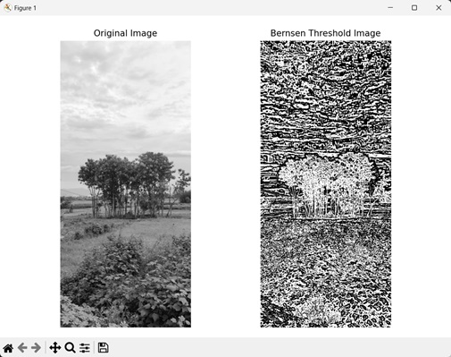
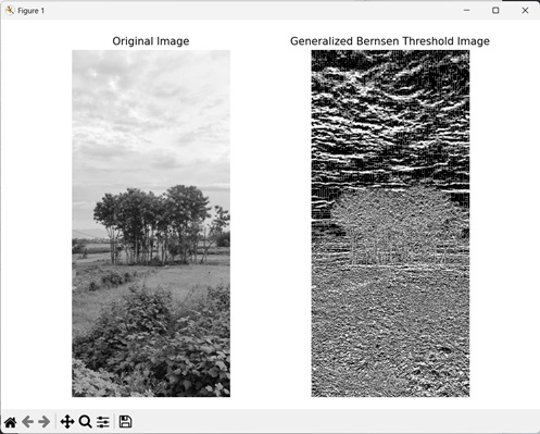
In this example, we are using mh.thresholding.gbernsen() function to apply generalized Bernsen local thresholding on an image.

import mahotas as mh
import numpy as np
import matplotlib.pyplot as mtplt
# Loading the image
image = mh.imread('nature.jpeg')
# Converting it to grayscale
image = mh.colors.rgb2gray(image)
# Creating a structuring element
structuring_element = np.array([[0, 0, 0],[0, 0, 0],[1, 1, 1]])
# Creating generalized Bernsen threshold image
threshold_image = mh.thresholding.gbernsen(image, structuring_element, 200,
128)
# Creating a figure and axes for subplots
fig, axes = mtplt.subplots(1, 2)
# Displaying the original image
axes[0].imshow(image, cmap='gray')
axes[0].set_title('Original Image')
axes[0].set_axis_off()
# Displaying the threshold image
axes[1].imshow(threshold_image, cmap='gray')
axes[1].set_title('Generalized Bernsen Threshold Image')
axes[1].set_axis_off()
# Adjusting spacing between subplots
mtplt.tight_layout()
# Showing the figures
mtplt.show()

Output

Output of the above code is as follows −

Bernsen Local Thresholding using Mean

We can apply Bernsen local thresholding using the mean value of the pixel intensities as the threshold value. It refers to the average intensity of an image and is calculated by summing the intensity value of all pixels and then dividing it by the total number of pixels.

In mahotas, we can do this by first finding the mean pixel intensities of all the pixels using the numpy.mean() function. Then, we define a window size to get the local neighborhood of a pixel.

Finally, we set the mean value as the threshold value by passing it to the to the contrast_threshold parameter of the bernsen() or gbernsen() function.

Example

Here, we are applying Bernsen local thresholding on an image where threshold value is the mean value of all pixel intensities.

import mahotas as mh
import numpy as np
import matplotlib.pyplot as mtplt
# Loading the image
image = mh.imread('nature.jpeg')
# Converting it to grayscale
image = mh.colors.rgb2gray(image)
# Calculating mean pixel value
mean = np.mean(image)
# Creating bernsen threshold image
threshold_image = mh.thresholding.bernsen(image, 15, mean)
# Creating a figure and axes for subplots
fig, axes = mtplt.subplots(1, 2)
# Displaying the original image
axes[0].imshow(image, cmap='gray')
axes[0].set_title('Original Image')
axes[0].set_axis_off()
# Displaying the threshold image
axes[1].imshow(threshold_image, cmap='gray')
axes[1].set_title('Bernsen Threshold Image')
axes[1].set_axis_off()
# Adjusting spacing between subplots
mtplt.tight_layout()
# Showing the figures
mtplt.show()

Output

After executing the above code, we get the following output −

Print Page