Mahotas - Daubechies Wavelet

Daubechies wavelets are perpendicular wavelets, which refer to mathematical functions that can represent an image using waves.

Daubechies wavelets have a non−zero value only within a finite interval and are characterized by a maximum number of vanishing moments.

Vanishing moments of a wavelet refers to the number of moments that is equal to zero. Moments are integrals (area under a curve) of the wavelet function multiplied by powers of x.

A wavelet with more vanishing moments better represents smooth signals, while a wavelet with fewer vanishing moments better represents signals with discontinuities.

Daubechies Wavelet in Mahotas

In Mahotas, we can apply Daubechies wavelet transformation on an image using the mahotas.daubechies() function.

It supports multiple Daubechies wavelets ranging from D2 to D20, where the integer represents the number of vanishing moments in a wavelet.

The transformations involve breaking the image into low−frequency (smooth features) and high−frequency coefficients (detailed features). This allows different frequencies of the image to be analyzed independently.

The mahotas.daubechies() function

The mahotas.daubechies() function takes a grayscale image as input, and returns the wavelet coefficients as a new image.

The wavelet coefficients are a tuple of arrays that correspond to the smooth and the detailed features of the image.

Syntax

Following is the basic syntax of the daubechies() function in mahotas −

mahotas.daubechies(f, code, inline=False)

Where,

f − It is the input image.
code − It specifies the type of wavelet to use, can be 'D2', 'D4',....., 'D20'.
inline (optional) − It specifies whether to return a new image or modify input image (default is False).

Example

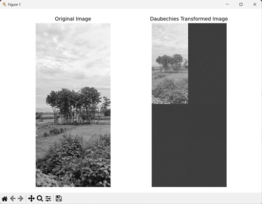
In the following example, we are applying Daubechies wavelet transformation on an image using the mh.daubechies() function.

import mahotas as mh
import numpy as np
import matplotlib.pyplot as mtplt
# Loading the image
image = mh.imread('nature.jpeg')
# Converting it to grayscale
image = mh.colors.rgb2gray(image)
# Applying Daubechies transformation
daubechies_transform = mh.daubechies(image, 'D20')
# Creating a figure and axes for subplots
fig, axes = mtplt.subplots(1, 2)
# Displaying the original image
axes[0].imshow(image, cmap='gray')
axes[0].set_title('Original Image')
axes[0].set_axis_off()
# Displaying the Daubechies transformed image
axes[1].imshow(daubechies_transform, cmap='gray')
axes[1].set_title('Daubechies Transformed Image')
axes[1].set_axis_off()
# Adjusting spacing between subplots
mtplt.tight_layout()
# Showing the figures
mtplt.show()

Output

Following is the output of the above code −

Multiple Daubechies Wavelets

Another way of applying Daubechies wavelet transformation is by using multiple Daubechies wavelets. Multiple Daubechies wavelets refers to a set of wavelets having different vanishing moments.

In mahotas, to apply multiple Daubechies wavelets we first create a list of different wavelets. Then, we traverse over each wavelet in the list.

Finally, we apply the different wavelets to the input image using the mh.daubechies() function.

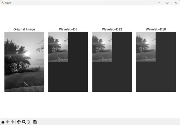
For example, let’s say we have a list of three wavelets − D6, D12, and D18. The three wavelets will have 6, 12, and 18 vanishing moments respectively.

Hence, three output images will be generated, each having a different Daubechies wavelet applied to it.

Example

In the example mentioned below, we are applying multiple Daubechies wavelets transformations on an image.

import mahotas as mh
import numpy as np
import matplotlib.pyplot as mtplt
# Loading the image
image = mh.imread('sun.png')
# Converting it to grayscale
image = mh.colors.rgb2gray(image)
# Creating list of multiple Daubechies wavelets
daubechies_wavelets = ['D6', 'D12', 'D18']
# Creating subplots to display images for each Daubechies wavelet
fig, axes = mtplt.subplots(1, len(daubechies_wavelets) + 1)
axes[0].imshow(image, cmap='gray')
axes[0].set_title('Original Image')
axes[0].set_axis_off()
# Applying Daubechies transformation for each Daubechies wavelet
for i, daubechies in enumerate(daubechies_wavelets):
   daubechies_transform = mh.daubechies(image, daubechies)
   axes[i + 1].imshow(daubechies_transform, cmap='gray')
   axes[i + 1].set_title(f'Wavelet={daubechies}')
   axes[i + 1].set_axis_off()
# Adjusting spacing between subplots
mtplt.tight_layout()
# Showing the figures
mtplt.show()

Output

Output of the above code is as follows −

Daubechies Wavelet on a Random Image

We can also perform Daubechies transformation by using Daubechies wavelets on a random image of two dimension.

A random two−dimensional image refers to an image having a random intensity value for each pixel. The intensity value can range from 0 (black) to 255 (white).

In mahotas, to perform Daubechies wavelet transformation on a random image, we first specify the dimensions (length and width) of the 2−D image.

Then, we pass these dimension along with the intensity range (0 to 255) to np.random.randint() function to create the random image. Since the channel value is not specified, the created image is a grayscale image.

After that, we apply Daubechies wavelet transformation by specifying the wavelet we want to use.

Example

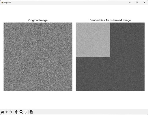
In here, we are applying Daubechies wavelet transformation on a randomly generated two−dimensional image.

import mahotas as mh
import numpy as np
import matplotlib.pyplot as mtplt
# Specifying the dimensions
length, width = 1000, 1000
# Creating a random two-dimensional image
image = np.random.randint(0, 256, (length, width))
# Applying Daubechies transformation
daubechies_transform = mh.daubechies(image, 'D2')
# Creating a figure and axes for subplots
fig, axes = mtplt.subplots(1, 2)
# Displaying the original image
axes[0].imshow(image, cmap='gray')
axes[0].set_title('Original Image')
axes[0].set_axis_off()
# Displaying the Daubechies transformed image
axes[1].imshow(daubechies_transform, cmap='gray')
axes[1].set_title('Daubechies Transformed Image')
axes[1].set_axis_off()
# Adjusting spacing between subplots
mtplt.tight_layout()
# Showing the figures
mtplt.show()

Output

After executing the above code, we get the following output −

Print Page