Mahotas - 2D Laplacian Filter

A Laplacian filter is used to detect edges and changes in intensity within an image. Mathematically, the Laplacian filter is defined as the sum of the second derivatives of the image in the x and y directions.

The second derivative provides information about the rate of change of intensity of each pixel.

The Laplacian filter emphasizes regions of an image where the intensity changes rapidly, such as edges and corners. It works by subtracting the average of the surrounding pixels from the center pixel, which gives a measure of the second derivative of intensity.

In 2D, the Laplacian filter is typically represented by a square matrix, often 3×3 or 5×5. Here's an example of a 3×3 Laplacian filter −

0  1  0
1 -4  1
0  1  0

2D Laplacian Filter in Mahotas

To apply the 2D Laplacian filter in mahotas, we can use the mahotas.laplacian_2D() function. Here is an overview of the working of the 2D Laplacian filter in Mahotas −

Input Image

The filter takes a grayscale input image.

Convolution

The Laplacian filter applies a convolution operation on the input image using a kernel. The kernel determines the weights applied to the neighboring pixels during convolution.
The convolution operation involves sliding the kernel over the entire image. At each pixel position, the Laplacian filter multiplies the corresponding kernel weights with the pixel values in the neighborhood and calculates the sum.

Laplacian Response

The Laplacian response is obtained by applying the Laplacian operator to the image.
It represents the intensity changes or discontinuities in the image, which are associated with edges.

The mahotas.laplacian_2D() function

The mahotas.laplacian_2D() function takes a grayscale image as input and performs a 2D laplacian operation on it. The resulting image highlights regions of rapid intensity changes, such as edges.

Syntax

Following is the basic syntax of the laplacian_2D() function in mahotas −

mahotas.laplacian_2D(array, alpha=0.2)

Where,

array − It is the input image.
alpha (optional) − It is a scalar value between 0 and 1 that controls the shape of Laplacian filter. A larger value of alpha increases the sensitivity of the Laplacian filter to the edges. The default value is 0.2.

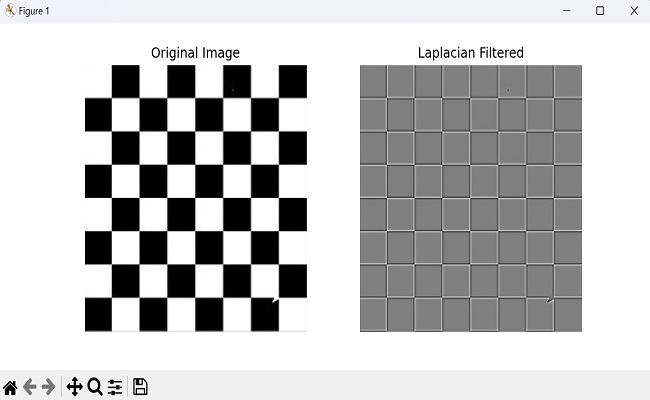
Example

Following is the basic example of detecting edges in an image using the laplacian_2D() function −

import mahotas as mh
import numpy as np
import matplotlib.pyplot as mtplt
image = mh.imread('picture.jpg', as_grey = True)
# Applying a laplacian filter
filtered_image = mh.laplacian_2D(image)
# Displaying the original image
fig, axes = mtplt.subplots(1, 2, figsize=(9, 4))
axes[0].imshow(image, cmap='gray')
axes[0].set_title('Original Image')
axes[0].axis('off')
# Displaying the laplacian filtered featured image
axes[1].imshow(filtered_image, cmap='gray')
axes[1].set_title('Laplacian Filtered')
axes[1].axis('off')
mtplt.show()

Output

After executing the above code, we get the following output −

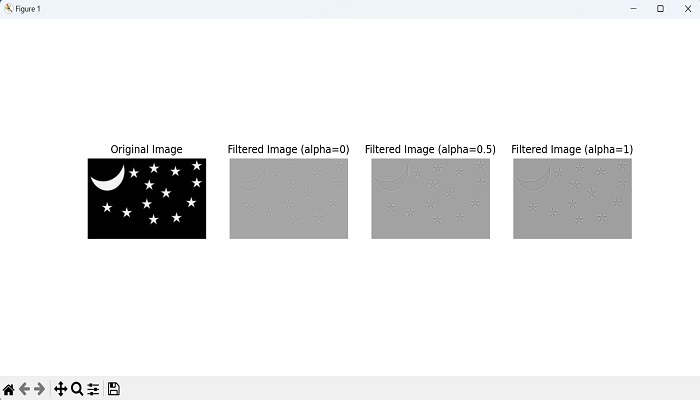
Scaling the Laplacian Response

By varying the alpha parameter, we can control the scale of the Laplacian response. A smaller alpha value, such as 0.2, produces a relatively subtle response, highlighting finer details and edges.

On the other hand, a larger alpha value, like 0.8, amplifies the response, making it more pronounced and emphasizing more prominent edges and structures.

Hence, we can use different alpha values in the laplacian filter to reflect the changes in edge detection.

Example

In here, we are using different alpha values in the laplacian filter to reflect the changes in edge detection −

import mahotas as mh
import matplotlib.pyplot as plt
# Load an example image
image = mh.imread('pic.jpg', as_grey=True)
# Apply the Laplacian filter with different alpha values
filtered_image_1 = mh.laplacian_2D(image, alpha=0)
filtered_image_2 = mh.laplacian_2D(image, alpha=0.5)
filtered_image_3 = mh.laplacian_2D(image, alpha=1)
# Display the original and filtered images with different scales
fig, axes = plt.subplots(1, 4, figsize=(12, 3))
axes[0].imshow(image, cmap='gray')
axes[0].set_title('Original Image')
axes[0].axis('off')
axes[1].imshow(filtered_image_1, cmap='gray')
axes[1].set_title('Filtered Image (alpha=0)')
axes[1].axis('off')
axes[2].imshow(filtered_image_2, cmap='gray')
axes[2].set_title('Filtered Image (alpha=0.5)')
axes[2].axis('off')
axes[3].imshow(filtered_image_3, cmap='gray')
axes[3].set_title('Filtered Image (alpha=1)')
axes[3].axis('off')
plt.show()

Output

Followng is the output of the above code −

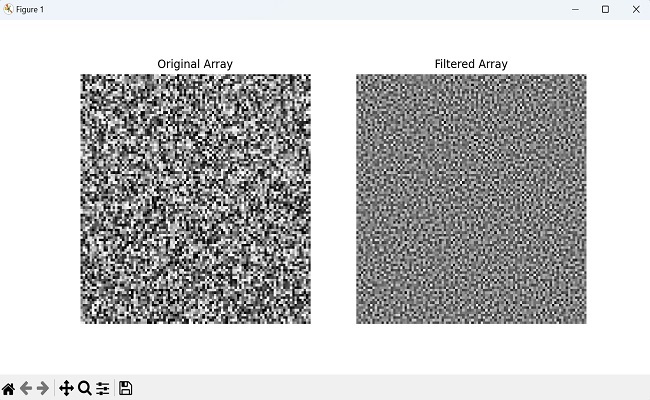
Using Randomly Generated Array

We can apply laplacian filter on a randomly generated array as well. To achieve this, first we need to create a random 2D array. We can create the array using the np.random.rand() function of the NumPy library.

This function generates values between 0 and 1, representing the pixel intensities of the array.

Next, we pass the randomly generated array to the mahotas.laplacian_2D() function. This function applies the Laplacian filter to the input array and returns the filtered array.

Example

Now, we are trying to apply laplacian filter to a randomly generated array −

import mahotas as mh
import numpy as np
import matplotlib.pyplot as plt
# Generate a random 2D array
array = np.random.rand(100, 100)
# Apply the Laplacian filter
filtered_array = mh.laplacian_2D(array)
# Display the original and filtered arrays
plt.figure(figsize=(10, 5))
plt.subplot(1, 2, 1)
plt.imshow(array, cmap='gray')
plt.title('Original Array')
plt.axis('off')
plt.subplot(1, 2, 2)
plt.imshow(filtered_array, cmap='gray')
plt.title('Filtered Array')
plt.axis('off')
plt.show()

Output

Output of the above code is as follows −

Print Page