Mahotas - Local Minima in Image

Local minima in an image refers to regions where the pixel intensity is the lowest within a local neighborhood. A local neighborhood consists of only immediate neighbors of a pixel; hence it uses only a portion of an image when identifying local minima.

An image can contain multiple local minima, each having different intensities. This happens because a region can have lower intensity than its neighboring regions, but it may not be the region with lowest intensity in the entire image.

Local Minima in Image in Mahotas

In Mahotas, we can find the local minima of an image using the mahotas.locmin() function. The local minima regions are found using regional minima, which refers to regions having lower intensity values than all their neighboring pixels in an image.

The mahotas.locmin() function

The 'mahotas.locmin()' function takes an image as input and finds the local minima regions. It returns a binary image where each local minima region is represented by 1. The function works in the following way to find local minima in an image −

It first applies a morphological erosion on the input image to find the regional minima points.
Next, it compares the eroded image with the original image. If the pixel intensity is lower in the original image, then the pixel represents a regional minima.
Finally, a binary array is generated where 1 corresponds to presence of local minima and 0 elsewhere.

Syntax

Following is the basic syntax of the locmin() function in mahotas −

mahotas.locmin(f, Bc={3x3 cross}, out={np.empty(f.shape, bool)})

Where,

f − It is the input grayscale image.
Bc (optional) − It is the structuring element used for connectivity.
out(optional) − It is the output array of Boolean data type (defaults to new array of same size as f).

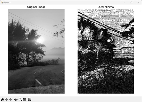
Example

In the following example, we are getting the local minima of an image using mh.locmin() function.

import mahotas as mh
import numpy as np
import matplotlib.pyplot as mtplt
# Loading the image
image = mh.imread('sun.png')
# Converting it to grayscale
image = mh.colors.rgb2gray(image)
# Getting the local minima
local_minima = mh.locmin(image)
# Creating a figure and axes for subplots
fig, axes = mtplt.subplots(1, 2)
# Displaying the original image
axes[0].imshow(image, cmap='gray')
axes[0].set_title('Original Image')
axes[0].set_axis_off()
# Displaying the local minima
axes[1].imshow(local_minima, cmap='gray')
axes[1].set_title('Local Minima')
axes[1].set_axis_off()
# Adjusting spacing between subplots
mtplt.tight_layout()
# Showing the figures
mtplt.show()

Output

Following is the output of the above code −

Using Custom Structuring Element

We can use a custom structuring element to get local minima of an image. A structuring element is a binary array of odd dimensions consisting of ones and zeroes that defines the connectivity pattern of the neighborhood pixels.

The ones indicate the neighboring pixels that are included in the connectivity analysis, while the zeros represent the neighbors that are excluded or ignored.

In mahotas, we can use custom structuring element to define the neighboring pixels of an image during local minima extraction. It allows us to find local minima regions as per our requirement.

To use a structuring element, we need to pass it to the Bc parameter of the locmin() function.

For example, let's consider the custom structuring element: [[1, 0, 0, 0, 1], [0, 1, 0, 1,0], [0, 0, 1, 0, 0], [0, 1, 0, 1, 1], [1, 0, 0, 1, 0]]. This structuring element implies vertical, horizontal, and diagonal connectivity.

It means that for each pixel in the image, only the pixels vertically, horizontally or diagonally above and below it is considered its neighbor during local minima extraction.

Example

In the example below, we are defining a custom structuring element to get the local minima of an image.

import mahotas as mh
import numpy as np
import matplotlib.pyplot as mtplt
# Loading the image
image = mh.imread('nature.jpeg')
# Converting it to grayscale
image = mh.colors.rgb2gray(image)
# Setting custom structuring element
struct_element = np.array([[1, 0, 0, 0, 1],
[0, 1, 0, 1, 0],
[0, 0, 1, 0, 0],
[0, 1, 0, 1, 1],
[1, 0, 0, 1, 0]])
# Getting the local minima
local_minima = mh.locmin(image, Bc=struct_element)
# Creating a figure and axes for subplots
fig, axes = mtplt.subplots(1, 2)
# Displaying the original image
axes[0].imshow(image, cmap='gray')
axes[0].set_title('Original Image')
axes[0].set_axis_off()
# Displaying the local minima
axes[1].imshow(local_minima, cmap='gray')
axes[1].set_title('Local Minima')
axes[1].set_axis_off()
# Adjusting spacing between subplots
mtplt.tight_layout()
# Showing the figures
mtplt.show()

Output

Output of the above code is as follows −

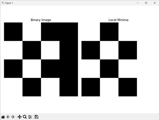
Using a Binary Image

We can also find the local minima in a binary image. A binary image is an image where each pixel is represented by a 1 or a 0, indicating either a foreground or background respectively. Binary images can be created using the array() function from the numpy library.

In mahotas, we can use the locmin() function to find local minima regions of a binary image. Since binary images consists of only 1’s and 0’s, the pixels having a value 1 will be considered local minima since the intensity of foreground pixels is less than background pixels.

For example, let’s assume a binary image is created from the following array: [[0, 1, 0, 0], [1, 0, 1, 0], [0, 1, 0, 0], [1, 0, 1, 0]]. Then the number of 1’s in an array will determine the number of local minima regions. Hence, the first array will have 1 local minima region, the second array will have 2 local minima regions and so on.

Example

Here, we are getting the local minima in a binary image.

import mahotas as mh
import numpy as np
import matplotlib.pyplot as mtplt
# Creating a binary image
binary_image = np.array([[0, 1, 0, 0],
[1, 0, 1, 0],
[0, 1, 0, 0],
[1, 0, 1, 0]], dtype=np.uint8)
# Getting the local minima
local_minima = mh.locmin(binary_image)
# Creating a figure and axes for subplots
fig, axes = mtplt.subplots(1, 2)
# Displaying the binary image
axes[0].imshow(binary_image, cmap='gray')
axes[0].set_title('Binary Image')
axes[0].set_axis_off()
# Displaying the local minima
axes[1].imshow(local_minima, cmap='gray')
axes[1].set_title('Local Minima')
axes[1].set_axis_off()
# Adjusting spacing between subplots
mtplt.tight_layout()
# Showing the figures
mtplt.show()

Output

After executing the above code, we get the following output −

Print Page