Mahotas - Loading Image as Grey

---

---

The grayscale images are a kind of black−and−white images or gray monochrome, consisting of only shades of gray. The contrast ranges from black to white, which is the weakest intensity to the strongest respectively.

The grayscale image only contains the brightness information and no color information. This is the reason of white being the maximum luminance (brightness) and black being the zero luminance, and everything in between consists shades of gray.

Loading Grayscale Images

In Mahotas, loading grayscale images involves reading an image file that only contains intensity values for each pixel. The resulting image is represented as a 2D array, where each element represents the intensity of a pixel.

Following is the basic syntax for loading grayscale Images in Mahotas −

mahotas.imread('image.file_format', as_grey=True)

Where, 'image.file_format' is the actual path and format of the image you want to load and 'as_grey=True' is passed as an argument to indicate that we want to load the image as grayscale.

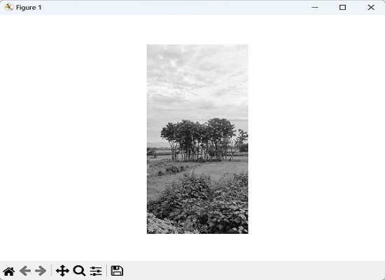
Example

Following is an example of loading a grayscale image in Mahotas −

import mahotas as ms
import matplotlib.pyplot as mtplt
# Loading grayscale image
grayscale_image = ms.imread('nature.jpeg', as_grey=True)
# Displaying grayscale image
mtplt.imshow(grayscale_image, cmap='gray')
mtplt.axis('off')
mtplt.show()

Output

After executing the above code, we get the output as shown below −

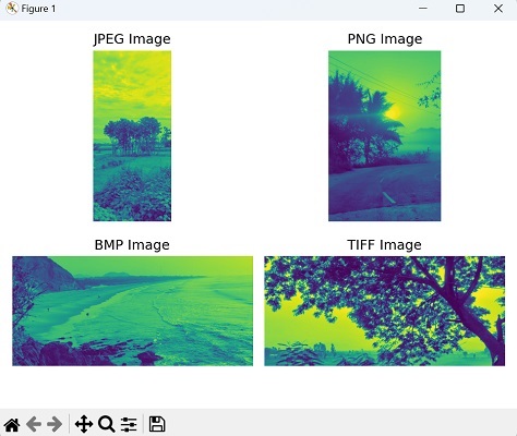
Loading Different Image Formats as Grayscale

The image format refers to the different file formats used to store and encode images digitally. Each format has its own specifications, characteristics, and compression methods.

Mahotas provides a wide range of image formats, including common formats like JPEG, PNG, BMP, TIFF, and GIF. We can pass the file path of a grayscale image in any of these formats to the imread() function.

Example

In this example, we demonstrate the versatility of Mahotas by loading grayscale images in different formats using the imread() function. Each loaded image is stored in a separate variable −

import mahotas as ms
import matplotlib.pyplot as mtplt
# Loading JPEG image
image_jpeg = ms.imread('nature.jpeg', as_grey = True)
# Loading PNG image
image_png = ms.imread('sun.png',as_grey = True)
# Loading BMP image
image_bmp = ms.imread('sea.bmp',as_grey = True)
# Loading TIFF image
image_tiff = ms.imread('tree.tiff',as_grey = True)
# Creating a figure and subplots
fig, axes = mtplt.subplots(2, 2)
# Displaying JPEG image
axes[0, 0].imshow(image_jpeg)
axes[0, 0].axis('off')
axes[0, 0].set_title('JPEG Image')
# Displaying PNG image
axes[0, 1].imshow(image_png)
axes[0, 1].axis('off')
axes[0, 1].set_title('PNG Image')
# Displaying BMP image
axes[1, 0].imshow(image_bmp)
axes[1, 0].axis('off')
axes[1, 0].set_title('BMP Image')
# Displaying TIFF image
axes[1, 1].imshow(image_tiff)
axes[1, 1].axis('off')
axes[1, 1].set_title('TIFF Image')
# Adjusting the spacing and layout
mtplt.tight_layout()
# Showing the figure
mtplt.show()

Output

The image displayed is as follows −

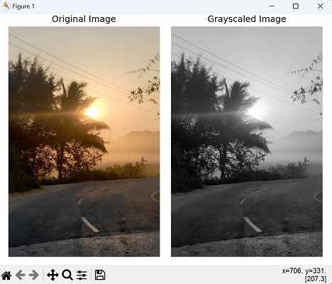
Using the Color Mode 'L'

The "L" color mode represents luminance, which is a measure of the brightness of a color. It is derived from the RGB (Red, Green, Blue) color model, in which the intensity values of the red, green and blue channels are combined to calculate the grayscale intensity. The "L" mode discards the color information and represents the image using only the grayscale intensity values.

To load image as grey by specifying the color mode as "L" in mahotas, we need to pass the parameter as_grey='L' to the imread() function.

Example

In here, we are loading a grayscale image and specifying the color mode as 'L' −

import mahotas as ms
import matplotlib.pyplot as mtplt
# Loading grayscale image
image = ms.imread('sun.png')
grayscale_image = ms.imread('sun.png', as_grey = 'L')
# Creating a figure and subplots
fig, axes = mtplt.subplots(1, 2)
# Displaying original image
axes[0].imshow(image)
axes[0].axis('off')
axes[0].set_title('Original Image')
# Displaying grayscale image
axes[1].imshow(grayscale_image, cmap='gray')
axes[1].axis('off')
axes[1].set_title('Grayscaled Image')
# Adjusting the spacing and layout
mtplt.tight_layout()
# Showing the figure
mtplt.show()

Output

Following is the output of the above code −