- Matplotlib - Home
- Matplotlib - Introduction
- Matplotlib - Vs Seaborn
- Matplotlib - Environment Setup
- Matplotlib - Anaconda distribution
- Matplotlib - Jupyter Notebook
- Matplotlib - Pyplot API
- Matplotlib - Simple Plot
- Matplotlib - Saving Figures
- Matplotlib - Markers
- Matplotlib - Figures
- Matplotlib - Styles
- Matplotlib - Legends
- Matplotlib - Colors
- Matplotlib - Colormaps
- Matplotlib - Colormap Normalization
- Matplotlib - Choosing Colormaps
- Matplotlib - Colorbars
- Matplotlib - Working With Text
- Matplotlib - Text properties
- Matplotlib - Subplot Titles
- Matplotlib - Images
- Matplotlib - Image Masking
- Matplotlib - Annotations
- Matplotlib - Arrows
- Matplotlib - Fonts
- Matplotlib - Font Indexing
- Matplotlib - Font Properties
- Matplotlib - Scales
- Matplotlib - LaTeX
- Matplotlib - LaTeX Text Formatting in Annotations
- Matplotlib - PostScript
- Matplotlib - Mathematical Expressions
- Matplotlib - Animations
- Matplotlib - Celluloid Library
- Matplotlib - Blitting
- Matplotlib - Toolkits
- Matplotlib - Artists
- Matplotlib - Styling with Cycler
- Matplotlib - Paths
- Matplotlib - Path Effects
- Matplotlib - Transforms
- Matplotlib - Ticks and Tick Labels
- Matplotlib - Radian Ticks
- Matplotlib - Dateticks
- Matplotlib - Tick Formatters
- Matplotlib - Tick Locators
- Matplotlib - Basic Units
- Matplotlib - Autoscaling
- Matplotlib - Reverse Axes
- Matplotlib - Logarithmic Axes
- Matplotlib - Symlog
- Matplotlib - Unit Handling
- Matplotlib - Ellipse with Units
- Matplotlib - Spines
- Matplotlib - Axis Ranges
- Matplotlib - Axis Scales
- Matplotlib - Axis Ticks
- Matplotlib - Formatting Axes
- Matplotlib - Axes Class
- Matplotlib - Twin Axes
- Matplotlib - Figure Class
- Matplotlib - Multiplots
- Matplotlib - Grids
- Matplotlib - Object-oriented Interface
- Matplotlib - PyLab module
- Matplotlib - Subplots() Function
- Matplotlib - Subplot2grid() Function
- Matplotlib - Anchored Artists
- Matplotlib - Manual Contour
- Matplotlib - Coords Report
- Matplotlib - AGG filter
- Matplotlib - Ribbon Box
- Matplotlib - Fill Spiral
- Matplotlib - Findobj Method
- Matplotlib - Hyperlinks
- Matplotlib - Image Thumbnail
- Matplotlib - Plotting with Keywords
- Matplotlib - Create Logo
- Matplotlib - Multipage PDF
- Matplotlib - Multiprocessing
- Matplotlib - Print Stdout
- Matplotlib - Compound Path
- Matplotlib - Sankey Class
- Matplotlib - MRI with EEG
- Matplotlib - Stylesheets
- Matplotlib - Background Colors
- Matplotlib - Basemap
Matplotlib Events
- Matplotlib - Event Handling
- Matplotlib - Close Event
- Matplotlib - Mouse Move
- Matplotlib - Click Events
- Matplotlib - Scroll Event
- Matplotlib - Keypress Event
- Matplotlib - Pick Event
- Matplotlib - Looking Glass
- Matplotlib - Path Editor
- Matplotlib - Poly Editor
- Matplotlib - Timers
- Matplotlib - Viewlims
- Matplotlib - Zoom Window
Matplotlib Widgets
- Matplotlib - Cursor Widget
- Matplotlib - Annotated Cursor
- Matplotlib - Button Widget
- Matplotlib - Check Buttons
- Matplotlib - Lasso Selector
- Matplotlib - Menu Widget
- Matplotlib - Mouse Cursor
- Matplotlib - Multicursor
- Matplotlib - Polygon Selector
- Matplotlib - Radio Buttons
- Matplotlib - RangeSlider
- Matplotlib - Rectangle Selector
- Matplotlib - Ellipse Selector
- Matplotlib - Slider Widget
- Matplotlib - Span Selector
- Matplotlib - Textbox
Matplotlib Plotting
- Matplotlib - Line Plots
- Matplotlib - Area Plots
- Matplotlib - Bar Graphs
- Matplotlib - Histogram
- Matplotlib - Pie Chart
- Matplotlib - Scatter Plot
- Matplotlib - Box Plot
- Matplotlib - Arrow Demo
- Matplotlib - Fancy Boxes
- Matplotlib - Zorder Demo
- Matplotlib - Hatch Demo
- Matplotlib - Mmh Donuts
- Matplotlib - Ellipse Demo
- Matplotlib - Bezier Curve
- Matplotlib - Bubble Plots
- Matplotlib - Stacked Plots
- Matplotlib - Table Charts
- Matplotlib - Polar Charts
- Matplotlib - Hexagonal bin Plots
- Matplotlib - Violin Plot
- Matplotlib - Event Plot
- Matplotlib - Heatmap
- Matplotlib - Stairs Plots
- Matplotlib - Errorbar
- Matplotlib - Hinton Diagram
- Matplotlib - Contour Plot
- Matplotlib - Wireframe Plots
- Matplotlib - Surface Plots
- Matplotlib - Triangulations
- Matplotlib - Stream plot
- Matplotlib - Ishikawa Diagram
- Matplotlib - 3D Plotting
- Matplotlib - 3D Lines
- Matplotlib - 3D Scatter Plots
- Matplotlib - 3D Contour Plot
- Matplotlib - 3D Bar Plots
- Matplotlib - 3D Wireframe Plot
- Matplotlib - 3D Surface Plot
- Matplotlib - 3D Vignettes
- Matplotlib - 3D Volumes
- Matplotlib - 3D Voxels
- Matplotlib - Time Plots and Signals
- Matplotlib - Filled Plots
- Matplotlib - Step Plots
- Matplotlib - XKCD Style
- Matplotlib - Quiver Plot
- Matplotlib - Stem Plots
- Matplotlib - Visualizing Vectors
- Matplotlib - Audio Visualization
- Matplotlib - Audio Processing
Matplotlib Useful Resources
Matplotlib - Spines
What are Spines?
In Matplotlib library spines refer to the borders or edges of a plot that frame the data area. These spines encompass the boundaries of the plot defining the area where data points are displayed. By default a plot has four spines such as top, bottom, left and right.
Manipulating spines in Matplotlib offers flexibility in designing the visual aspects of a plot by allowing for a more tailored and aesthetically pleasing presentation of data.
Key Characteristics of Spines
The following are the characteristics of spines.
Borders of the Plot − Spines form the borders of the plot area enclose the region where data is visualized.
Configurable Properties − Each spine top, bottom, left, and right can be customized individually by allowing adjustments to their appearance, color, thickness and visibility.
Visibility Control − Spines can be made visible or hidden to modify the appearance of the plot.
Uses of Spines
Plot Customization − Spines allow customization of the plot's appearance enabling adjustments to the plot's boundaries and style.
Aesthetics and Visualization − Customizing spines can enhance the aesthetics of the plot and draw attention to specific areas of interest.
Types of spines
Now lets see the each and every spine available in a plot in detail.
Top Spine
The Top spine refers to the horizontal line at the top of the plot area that corresponds to the upper boundary of the y-axis. It's one of the four spines such as top, bottom, left and right that form the borders around the plot.
Characteristics of the Top Spine
Boundary Line − The top spine represents the upper boundary of the plot area along the y-axis.
Default Visibility − By default the top spine is visible in Matplotlib plots.
Customization − Similar to other spines the top spine can be customized in terms of its visibility, color, linestyle and linewidth.
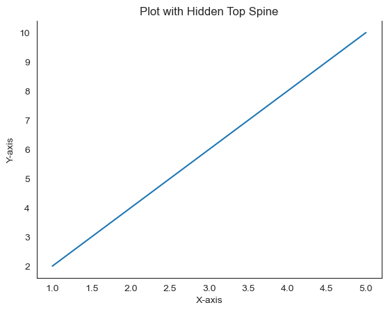
Example - Removing Top Spine
In this example ax.spines['top'].set_visible(False) hides the top spine by removing the upper boundary of the plot area along the y-axis.
import matplotlib.pyplot as plt

# Creating a simple plot
x = [1, 2, 3, 4, 5]
y = [2, 4, 6, 8, 10]
plt.plot(x, y)

# Accessing and modifying the top spine
ax = plt.gca()  # Get the current axes
ax.spines['top'].set_visible(False)  # Hide the top spine
plt.xlabel('X-axis')
plt.ylabel('Y-axis')
plt.title('Plot with Hidden Top Spine')
plt.show()
Output
Use Cases for Modifying the Top Spine
Aesthetic Control − Customizing the visibility, color or style of the top spine can improve the appearance or match specific design requirements.
Adjusting Plot Boundaries − Hiding the top spine might be useful when the plot doesn't require an upper boundary or when creating specific visual effects.
Bottom Spine
In Matplotlib the bottom spine refers to the horizontal line that forms the bottom border of the plot area corresponding to the x-axis.
Characteristics of the Bottom Spine
Association with x-axis − The bottom spine represents the border of the plot along the x-axis defining the lower boundary of the plot area.
Customization − Similar to other spines the bottom spine can be customized in terms of its visibility, color, line style, thickness and position.
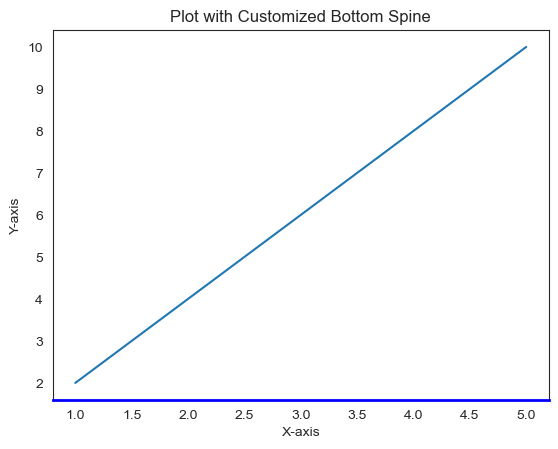
Example - Customizing the Bottom Spine
In this example by using ax.spines['bottom'].set_color('blue') changes the color of the bottom spine to blue, ax.spines['bottom'].set_linewidth(2) sets the thickness of the bottom spine to 2 and ax.spines['bottom'].set_visible(True) ensures the bottom spine is visible if in case it was hidden.
import matplotlib.pyplot as plt

# Creating a simple plot
x = [1, 2, 3, 4, 5]
y = [2, 4, 6, 8, 10]
plt.plot(x, y)

# Accessing and customizing the bottom spine
ax = plt.gca()  # Get the current axes
ax.spines['bottom'].set_color('blue')  # Change the color of the bottom spine to blue
ax.spines['bottom'].set_linewidth(2)  # Set the thickness of the bottom spine to 2
ax.spines['bottom'].set_visible(True)  # Make the bottom spine visible (if previously hidden)
plt.xlabel('X-axis')
plt.ylabel('Y-axis')
plt.title('Plot with Customized Bottom Spine')
plt.show()
Output
Use Cases for Bottom Spine Customization
Emphasizing Axes − By customizing the bottom spine can draw attention to the x-axis and enhance the plot's aesthetics.
Highlighting Plot Boundaries − By adjusting the appearance of the bottom spine can help in delineating the plot area and improving its clarity.
Left Spine
In Matplotlib the left spine refers to the vertical line that forms the left border of the plot area, corresponding to the y-axis.
Characteristics of the Left Spine
Association with y-axis − The left spine represents the border of the plot along the y-axis defining the left boundary of the plot area.
Customization − The customization of the left spine is similar to the other pines which can be customized by color, visibility, border width etc.
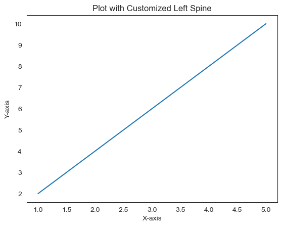
Example - Customizing the Left Spine
In this example ax.spines['left'].set_color('green') changes the color of the left spine to green, ax.spines['left'].set_linewidth(2) sets the thickness of the left spine to 2 and ax.spines['left'].set_visible(False) ensures the left spine is invisible if in case it was visible.
import matplotlib.pyplot as plt

# Creating a simple plot
x = [1, 2, 3, 4, 5]
y = [2, 4, 6, 8, 10]
plt.plot(x, y)

# Accessing and customizing the left spine
ax = plt.gca()  # Get the current axes
ax.spines['left'].set_color('green')  # Change the color of the left spine to green
ax.spines['left'].set_linewidth(2)  # Set the thickness of the left spine to 2
ax.spines['left'].set_visible(False)  # Make the left spine invisible (if previously visible)
plt.xlabel('X-axis')
plt.ylabel('Y-axis')
plt.title('Plot with Customized Left Spine')
plt.show()
Output
Right Spine
In Matplotlib the right spine represents the vertical line forming the right border of the plot area corresponding to the y-axis on the right side.
Characteristics of the Right Spine
Associated with y-axis − The right spine defines the right border of the plot along the y-axis representing, the y-axis on the right side of the plot.
Customization − Similar to other spines the right spine can be customized in terms of its visibility, color, line style, thickness and position.
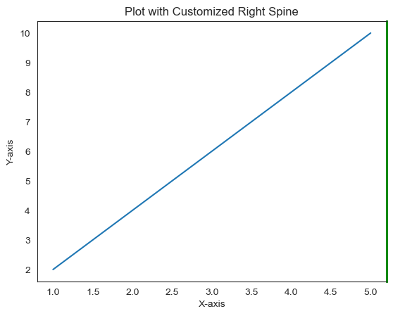
Example - Customizing the Right Spine
In this example we are using ax.spines['right'] to customize the right spine to the plot.
import matplotlib.pyplot as plt

# Creating a simple plot
x = [1, 2, 3, 4, 5]
y = [2, 4, 6, 8, 10]
plt.plot(x, y)

# Accessing and customizing the right spine
ax = plt.gca()  # Get the current axes
ax.spines['right'].set_color('green')  # Change the color of the right spine to green
ax.spines['right'].set_linewidth(2)  # Set the thickness of the right spine to 2
ax.spines['right'].set_visible(True)  # Make the right spine visible (if previously hidden)
plt.xlabel('X-axis')
plt.ylabel('Y-axis')
plt.title('Plot with Customized Right Spine')
plt.show()
Output
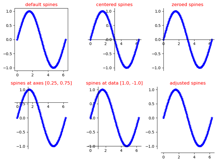
Example - Customize spines of Matplotlib figures
In this example we are creating six figures to see and customize the spines for it.
#First import the required libraries for the workbook.
import numpy as np
import matplotlib.pyplot as plt

#draw graph for sines
theta = np.linspace(0, 2*np.pi, 128)
y = np.sin(theta)
fig = plt.figure(figsize=(8,6))

#Define the axes with default spines
ax1 = fig.add_subplot(2, 3, 1)
ax1.plot(theta, np.sin(theta), 'b-*')
ax1.set_title('default spines')

#Define the function to plot the graph
def plot_graph(axs, title, lposition, bposition):
   ax = fig.add_subplot(axs)
   ax.plot(theta, y, 'b-*')
   ax.set_title(title)
   ax.spines['left'].set_position(lposition)
   ax.spines['right'].set_visible(False)
   ax.spines['bottom'].set_position(bposition)
   ax.spines['top'].set_visible(False)
   ax.xaxis.set_ticks_position('bottom')
   ax.yaxis.set_ticks_position('left')

#plot 3 graphs
plot_graph(232, 'centered spines', 'center', 'center')
plot_graph(233, 'zeroed spines', 'zero', 'zero')
plot_graph(234, 'spines at axes [0.25, 0.75]', ('axes', 0.25),('axes', 0.75))
plot_graph(235, 'spines at data [1.0, -1.0]', ('data', 1.0),('data', -1.0))
plot_graph(236, 'adjusted spines', ('outward', 10), ('outward', 10))

#fit the plot in the grid and display.
plt.tight_layout()
plt.show()
Output