Matplotlib - Latex

Quiz

What is LaTeX?

LaTeX is a typesetting system widely used for producing scientific and technical documents, particularly in disciplines such as mathematics, physics, computer science, engineering and academic writing. It's highly regarded for its superior typesetting of complex mathematical equations, scientific notations, and structured text formatting.

Key Aspects of LaTeX

The below are the key aspects of LaTeX.

Markup Language: LaTeX is a markup language, meaning it uses commands and tags to format text rather than WYSIWYG which is abbreviated as What You See Is What You Get editors. Users write plain text with embedded commands that specify the structure and formatting.
High-Quality Typesetting: LaTeX excels in producing professional-looking documents with precise typographical and typesetting features. It handles complex structures like mathematical formulas, tables, bibliographies and cross-references exceptionally well.
Package System: LaTeX offers a vast array of packages that extend its functionality for specific tasks or document types, providing templates, styles and additional features.
Free and Open Source: LaTeX is free to use and is supported by a strong open-source community by ensuring continuous development and a rich ecosystem of packages and resources.
Components of LaTeX: The LaTex of matplotlib library have the following components. Let's see each of them in detail.
Document Class: The document class specifies the type of document being created and defines its overall structure, layout and formatting. It acts as a template that sets the style and behaviour for the entire document. Different document classes are available to suit various types of documents such as articles, reports, books, presentations and more.
Preamble: In LaTeX the preamble is the section of the document that precedes the main content and the \begin{document} command. It is where we define the document settings, load packages, set parameters and configure global settings that apply to the entire document. The preamble acts as a setup area where we prepare LaTeX for processing the main body of the document.
Document Body: The document body in LaTeX is the main section where the content of our document resides. It starts after the preamble and the \begin{document} command and continues until the \end{document} command. This section includes the actual text, sections, subsections, equations, figures, tables and any other elements that constitute the core content of the document.

Advantages of LaTeX

The following are the advantages of LaTex −

Quality Typesetting: Produces high-quality output, especially for scientific and technical documents.
Cross-Referencing: Simplifies referencing and cross-referencing of equations, figures, tables, and sections.
Version Control: Facilitates version control and collaboration through plain text-based files.
Customization: Allows extensive customization of document styles, layouts and formatting.

Disadvantages of LaTeX

The following are the disadvantages of LaTex −

Learning Curve: Requires learning its syntax and commands which can be daunting for beginners.
Limited WYSIWYG: Lack of immediate visual feedback (WYSIWYG) might be challenging for some users accustomed to graphical editors.

Usage of LaTeX

Following is the usage of Latex −

Academic Writing: Academic papers, theses, dissertations
Scientific: Scientific reports, articles, and journals
Technical Documents: Technical documentation, manuals
Presentations: Presentations using tools like Beamer

Basic document structure of the LaTex

Following is the basic document structure of LaTeX. It defines a basic article document with a hierarchical structure comprising a section and a subsection.

\documentclass{article}
\begin{document}
\section{Introduction}
This is a simple LaTeX document.
\subsection{Subsection}
Some text in a subsection.
\end{document}

Writing our own LaTeX preamble

To write our own LaTeX preamble in Matplotlib we can use this example as reference.

Example 1

import numpy as np
from matplotlib import pyplot as plt
plt.rcParams["figure.figsize"] = [7.50, 3.50]
plt.rcParams["figure.autolayout"] = True
x = np.linspace(-10, 10, 100)
y = np.exp(x)
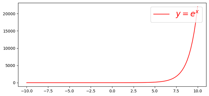
plt.plot(x, y, color='red', label="$y=e^{x}$")
plt.legend(loc='upper right')
plt.show()

Output

This will generate the following output −

Example 2

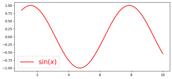
In this example we are using the Latex formula in the legend of a plot inside a .py file.

import numpy as np
import matplotlib.pyplot as plt
plt.rcParams["figure.figsize"] = [7.50, 3.50]
plt.rcParams["figure.autolayout"] = True
x = np.linspace(1, 10, 1000)
y = np.sin(x)
plt.plot(x, y, label=r'$\sin (x)$', c="red", lw=2)
plt.legend()
plt.show()

Output

This will generate the following output −

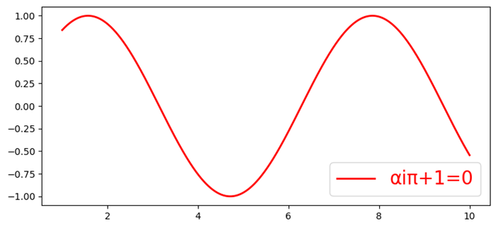
Put a little more complex equation in the label, for example, label=r'i+1=0'. Now look at the legend at the top-right corner of the plot.

Example 3

import numpy as np
import matplotlib.pyplot as plt
plt.rcParams["figure.figsize"] = [7.50, 3.50]
plt.rcParams["figure.autolayout"] = True
x = np.linspace(1, 10, 1000)
y = np.sin(x)
plt.plot(x, y, label=r'$\sin (x)$', c="red", lw=2)
plt.legend(r'i+1=0')
plt.show()

Output

This will generate the following output −

Rendering Mathematical Expressions

Rendering mathematical expressions in LaTeX involves using LaTeX syntax to write mathematical equations, symbols and formulas. LaTeX provides a comprehensive set of commands and notation to create complex mathematical expressions with precision and clarity.

Importance of LaTeX for Mathematics

Precision and Clarity: LaTeX allows precise typesetting of mathematical notation and symbols.
Consistency: Maintains consistency in formatting across mathematical documents.
Publication-Quality: Produces high-quality mathematical expressions suitable for academic and scientific publications.
LaTeX's support for mathematical typesetting makes it a preferred choice for researchers, mathematicians, scientists and academics when writing technical or mathematical documents that require accurate and well-formatted mathematical notation.

LaTeX for Mathematical Expressions

The below are the components of LaTex in Mathematical Expressions.

Inline Math Mode: Inline math mode in LaTeX is used to include mathematical expressions within the text of a document. We can use inline math mode by enclosing the mathematical expression between a pair of single dollar signs $...$.
Using the inline math mode: In this example the mathematical expression `\frac{-b \pm \sqrt{b^2 - 4ac}}{2a}` is included within the text using inline math mode. The result is that the mathematical expression is rendered within the line of text.

Example

Following is an example −

import matplotlib.pyplot as plt
equation = r'$x = \frac{{-b \pm \sqrt{{b^2 - 4ac}}}}{{2a}}$'
plt.text(0.5, 0.5, equation, fontsize=12, ha='center')
plt.axis('off')
plt.show()

This will generate the following output −

Display Math Mode

Display math mode in LaTeX is used to showcase mathematical expressions in a separate block, centered and distinct from the surrounding text. It's commonly used for larger or stand-alone equations that deserve prominence in a document.

To use display math mode in LaTeX we have several options let's see them one by one.

Double Dollar Sign `$$...$$`

Enclose the mathematical expression between $$ symbols for displayed equations. In the following example we are displaying the given input equation by using the $$..$$ −

Example

$$
   f(x) = \int_{a}^{b} g(x) \, dx
$$

Output

This will generate the following output −

The 'equation' Environment

Use the 'equation' environment to create a numbered equation.

Example

\begin{equation}
   f(x) = \int_{a}^{b} g(x) \, dx
   \end{equation}

Output

This will generate the following output −

Note: The above code lines can be executed in the Jupyter Notebook markdown mode.

Symbols and Operators

In LaTeX we can use a wide range of symbols and operators to represent mathematical notation, expressions and operations. Here are some commonly used symbols and operators along with their LaTeX commands.

Greek Letters: Alpha: `\alpha`, Beta: `\beta`, Gamma: `\gamma`, Delta: `\delta` and so on.
Arithmetic Operators: Plus: `+`, Minus: `-`, Multiplication: `\times` or `*`, Division: `\div` or `/`
Relations and Comparisons: Equals: `=`, Not equals: `\neq`, Less than: `<`, Greater than: `>` and so on.
Set Theory: Union: `\cup`, Intersection: `\cap`, Subset: `\subset`, Superset: `\supset` and so on
Calculus and Limits: Integral: `\int`, Summation: `\sum`, Limit: `\lim`, Derivative: `\frac{dy}{dx}`
Functions: Sine: `\sin`, Cosine: `\cos`, Tangent: `\tan`, Logarithm: `\log`, Exponential: `\exp`
Roots and Exponents: Square root: `\sqrt{x}`, Exponent: `x^2`, Subscript: `x_1`, Superscript: `x^i`

Other Notations

Fractions: `\frac{numerator}{denominator}`
Matrices: `bmatrix`, `pmatrix`, `vmatrix`, etc., using the `amsmath` package
Special Symbols: For example, `\infty` for infinity, `\emptyset` for an empty set, etc.

Example

In this example we are using the $..$, to display the symbols and operators in the LaTex of matplotlib library.

import matplotlib.pyplot as plt
import matplotlib as mpl
equation = r'$(\alpha + \beta = \gamma \times \delta)$'
plt.figure(figsize=(6, 3))
plt.text(0.5, 0.5, equation, fontsize=12, ha='center', va='center')
plt.axis('off')
plt.show()

This will display the following equation −

By utilizing these LaTeX commands for symbols and operators we can create complex mathematical expressions with precision and clarity in our LaTeX documents.

Fractions

In LaTeX we can easily create fractions, subscripts and superscripts to represent mathematical expressions using specific commands and notation.

To create fractions we can use the `\frac{numerator}{denominator}` command. In this example we are creating the fraction \frac{3}{4} .

Example

import matplotlib.pyplot as plt
import matplotlib as mpl
equation = r'The fraction is $\frac{3}{4}$'
plt.figure(figsize=(6, 3))
plt.text(0.5, 0.5, equation, fontsize=12, ha='center', va='center')
plt.axis('off')
plt.show()

Output

This will generate the following equation −

Matrices and Arrays

In LaTeX matrices and arrays are used to represent data in matrix form or to display sets of equations. The array environment is the basic structure for creating matrices and arrays in LaTeX while the matrix environments provided by the amsmath package offer additional functionality and easier syntax for matrices.

Creating Matrices and Arrays

Here are we are creating the arrays and matrices using respective environments.

Using 'array' Environment

The 'array' environment allows us to create matrices or arrays in LaTeX.

Example

\[
\begin{array}{ccc}
1 & 2 & 3 \\
4 & 5 & 6 \\
7 & 8 & 9 \\
\end{array}
\]

Output

This will generate the following equation −

Note: The above code lines can be executed in the Jupyter Notebook markdown mode.

Using 'amsmath' Package's 'matrix' Environments

The amsmath package provides convenient matrix environments such as matrix, pmatrix, bmatrix, Bmatrix, vmatrix, Vmatrix which simplify the creation of matrices.

Example

\[
\begin{matrix}
1 & 2 & 3 \\
4 & 5 & 6 \\
7 & 8 & 9 \\
\end{matrix}
\]

Output

This will generate the following equation −

Note: The above code lines can be executed in the Jupyter Notebook markdown mode.

Matrix Formatting

Here are going to align the columns of the matrix using the LaTex. In matrices or arrays we can specify column alignment using c for centered, l for left-aligned and r for right-aligned columns within the array environment.

The below is the example of applying the column alignment on a matrix.

Example

\[
\begin{array}{ccc}
1 & 222 & 3 \\
4 & 55555 & 6 \\
7 & 888 & 999999 \\
\end{array}
\]

Output

This will generate the following equation −

Note: The above code lines can be executed in the Jupyter Notebook markdown mode.

Additional Notes

Matrices and arrays in LaTeX are enclosed within the \[ ... \] or equation environment to display them as standalone equations.
The & symbol separates elements within a row and \\ starts a new row.

LaTeX provides versatile tools for displaying matrices and arrays allowing us to represent mathematical data or equations in matrix form with various alignments and configurations. LaTeX enables the creation of matrices and arrays for mathematical notation.

Example

\begin{bmatrix}
1 & 2 \\
3 & 4
\end{bmatrix}

Output

This will generate the following equation −

Note: The above code lines can be executed in the Jupyter Notebook markdown mode.

Special Functions

LaTeX supports notation for special functions like trigonometric functions, logarithms, etc.

Example

import matplotlib.pyplot as plt

# LaTeX code for the bold text
bold_text = r'$\sin(\theta), \log(x), \lim_{x \to \infty} f(x)$'

# Create a figure and display the bold text
plt.figure(figsize=(6, 3))
plt.text(0.5, 0.5, bold_text, fontsize=12, ha='center', va='center')
plt.axis('off')
plt.show()

Output

Remove random unwanted space in LaTeX-style maths

LaTeX ignores the spaces you type and uses spacing the way it's done in mathematics texts. You can use the following four commands in case you want a different spacing style.

\;: thick space
\:: medium space
\,: a thin space
\!: a negative thin space

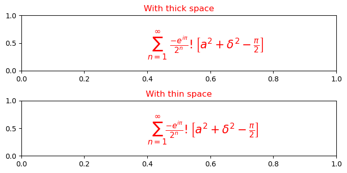
To remove random unwanted space in LaTeX-style maths in matplotlib plot we can use "\!" which will reduce the extra spacing.

The below is the example of applying the column alignment on a matrix.

Example

from matplotlib import pyplot as plt
plt.rcParams["figure.figsize"] = [7.00, 3.50]
plt.rcParams["figure.autolayout"] = True
plt.subplot(211)
plt.text(0.4, 0.4, r'$\sum_{n=1}^{\infty}\; \frac{-e^{i\pi}}{2^n}!\left[a^2+\delta ^2- \frac{\pi}{2} \right ]$', fontsize=16, color='r')
plt.title("With thick space")
plt.subplot(212)
plt.text(0.4, 0.4, r'$\sum_{n=1}^{\infty}\! \frac{-e^{i\pi}}{2^n}!\left[a^2+\delta ^2- \frac{\pi}{2} \right ]$', fontsize=16, color='r')
plt.title("With thin space")
plt.show()

Output

This will generate the following equation −

Notice the difference in spacing after the " (sigma)" symbol. In the first case, we have used thick space (\;) and in the second case, we have used the thin space (\!) to reduce extra spacing.

Print Page