- Python XlsxWriter - Home
- Python XlsxWriter - Overview
- Python XlsxWriter - Environment Setup
- Python XlsxWriter - Hello World
- Python XlsxWriter - Important classes
- Python XlsxWriter - Cell Notation & Ranges
- Python XlsxWriter - Defined Names
- Python XlsxWriter - Formula & Function
- Python XlsxWriter - Date and Time
- Python XlsxWriter - Tables
- Python XlsxWriter - Applying Filter
- Python XlsxWriter - Fonts & Colors
- Python XlsxWriter - Number Formats
- Python XlsxWriter - Border
- Python XlsxWriter - Hyperlinks
- Python XlsxWriter - Conditional Formatting
- Python XlsxWriter - Adding Charts
- Python XlsxWriter - Chart Formatting
- Python XlsxWriter - Chart Legends
- Python XlsxWriter - Bar Chart
- Python XlsxWriter - Line Chart
- Python XlsxWriter - Pie Chart
- Python XlsxWriter - Sparklines
- Python XlsxWriter - Data Validation
- Python XlsxWriter - Outlines & Grouping
- Python XlsxWriter - Freeze & Split Panes
- Python XlsxWriter - Hide/Protect Worksheet
- Python XlsxWriter - Textbox
- Python XlsxWriter - Insert Image
- Python XlsxWriter - Page Setup
- Python XlsxWriter - Header & Footer
- Python XlsxWriter - Cell Comments
- Python XlsxWriter - Working with Pandas
- Python XlsxWriter - VBA Macro
Python XlsxWriter - Quick Guide
Python XlsxWriter - Overview
XlsxWriter is a Python module for creating spreadsheet files in Excel 2007 (XLSX) format that uses open XML standards. XlsxWriter module has been developed by John McNamara. Its earliest version (0.0.1) was released in 2013. The latest version 3.0.2 was released in November 2021. The latest version requires Python 3.4 or above.
XlsxWriter Features
Some of the important features of XlsxWriter include −
Files created by XlsxWriter are 100% compatible with Excel XLSX files.
XlsxWriter provides full formatting features such as Merged cells, Defined names, conditional formatting, etc.
XlsxWriter allows programmatically inserting charts in XLSX files.
Autofilters can be set using XlsxWriter.
XlsxWriter supports Data validation and drop-down lists.
Using XlsxWriter, it is possible to insert PNG/JPEG/GIF/BMP/WMF/EMF images.
With XlsxWriter, Excel spreadsheet can be integrated with Pandas library.
XlsxWriter also provides support for adding Macros.
XlsxWriter has a Memory optimization mode for writing large files.
Python XlsxWriter - Environment Setup
Installing XlsxWriter using PIP
The easiest and recommended method of installing XlsxWriter is to use PIP installer. Use the following command to install XlsxWriter (preferably in a virtual environment).
pip3 install xlsxwriter
Installing from a Tarball
Another option is to install XlsxWriter from its source code, hosted at https://github.com/jmcnamara/XlsxWriter/. Download the latest source tarball and install the library using the following commands −
$ curl -O -L http://github.com/jmcnamara/XlsxWriter/archive/main.tar.gz

$ tar zxvf main.tar.gz
$ cd XlsxWriter-main/
$ python setup.py install
Cloning from GitHub
You may also clone the GitHub repository and install from it.
$ git clone https://github.com/jmcnamara/XlsxWriter.git

$ cd XlsxWriter
$ python setup.py install
To confirm that XlsxWriter is installed properly, check its version from the Python prompt −
>>> import xlsxwriter
>>> xlsxwriter.__version__
'3.0.2'
Python XlsxWriter - Hello World
Getting Started
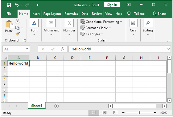
The first program to test if the module/library works correctly is often to write Hello world message. The following program creates a file with .XLSX extension. An object of the Workbook class in the xlsxwriter module corresponds to the spreadsheet file in the current working directory.
wb = xlsxwriter.Workbook('hello.xlsx')
Next, call the add_worksheet() method of the Workbook object to insert a new worksheet in it.
ws = wb.add_worksheet()
We can now add the Hello World string at A1 cell by invoking the write() method of the worksheet object. It needs two parameters: the cell address and the string.
ws.write('A1', 'Hello world')
Example
The complete code of hello.py is as follows −
import xlsxwriter
wb = xlsxwriter.Workbook('hello.xlsx')
ws = wb.add_worksheet()
ws.write('A1', 'Hello world')
wb.close()
Output
After the above code is executed, hello.xlsx file will be created in the current working directory. You can now open it using Excel software.
Python XlsxWriter - Important Classes
The XlsxWriter library comprises of following classes. All the methods defined in these classes allow different operations to be done programmatically on the XLSX file. The classes are −
- Workbook class
- Worksheet class
- Format class
- Chart class
- Chartsheet class
- Exception class
Workbook Class
This is the main class exposed by the XlsxWriter module and it is the only class that you will need to instantiate directly. It represents the Excel file as it is written on a disk.
wb=xlsxwriter.Workbook('filename.xlsx')
The Workbook class defines the following methods −
| Sr.No | Workbook Class & Description |
|---|---|
| 1 | add_worksheet() Adds a new worksheet to a workbook. |
| 2 | add_format() Used to create new Format objects which are used to apply formatting to a cell. |
| 3 | add_chart() Creates a new chart object that can be inserted into a worksheet via the insert_chart() Worksheet method |
| 4 | add_chartsheet() Adds a new chartsheet to a workbook. |
| 5 | close() Closes the Workbook object and write the XLSX file. |
| 6 | define_name() Creates a defined name in the workbook to use as a variable. |
| 7 | add_vba_project() Used to add macros or functions to a workbook using a binary VBA project file. |
| 8 | worksheets() Returns a list of the worksheets in a workbook. |
Worksheet Class
The worksheet class represents an Excel worksheet. An object of this class handles operations such as writing data to cells or formatting worksheet layout. It is created by calling the add_worksheet() method from a Workbook() object.
The Worksheet object has access to the following methods −
write() |
Writes generic data to a worksheet cell. Parameters −
Returns −
|
write_string() |
Writes a string to the cell specified by row and column. Parameters −
Returns −
|
write_number() |
Writes numeric types to the cell specified by row and column. Parameters −
Returns −
|
write_formula() |
Writes a formula or function to the cell specified by row and column. Parameters −
Returns −
|
insert_image() |
Used to insert an image into a worksheet. The image can be in PNG, JPEG, GIF, BMP, WMF or EMF format. Parameters −
Returns −
|
insert_chart() |
Used to insert a chart into a worksheet. A chart object is created via the Workbook add_chart() method. Parameters −
|
conditional_format() |
Used to add formatting to a cell or range of cells based on user-defined criteria. Parameters −
Returns −
|
add_table() |
Used to group a range of cells into an Excel Table. Parameters −
|
autofilter() |
Set the auto-filter area in the worksheet. It adds drop down lists to the headers of a 2D range of worksheet data. User can filter the data based on simple criteria. Parameters −
|
Format Class
Format objects are created by calling the workbook add_format() method. Methods and properties available to this object are related to fonts, colors, patterns, borders, alignment and number formatting.
Font formatting methods and properties −
| Method Name | Description | Property |
|---|---|---|
| set_font_name() | Font type | 'font_name' |
| set_font_size() | Font size | 'font_size' |
| set_font_color() | Font color | 'font_color' |
| set_bold() | Bold | 'bold' |
| set_italic() | Italic | 'italic' |
| set_underline() | Underline | 'underline' |
| set_font_strikeout() | Strikeout | 'font_strikeout' |
| set_font_script() | Super/Subscript | 'font_script' |
Alignment formatting methods and properties
| Method Name | Description | Property |
|---|---|---|
| set_align() | Horizontal align | 'align' |
| set_align() | Vertical align | 'valign' |
| set_rotation() | Rotation | 'rotation' |
| set_text_wrap() | Text wrap | 'text_wrap' |
| set_reading_order() | Reading order | 'reading_order' |
| set_text_justlast() | Justify last | 'text_justlast' |
| set_center_across() | Center across | 'center_across' |
| set_indent() | Indentation | 'indent' |
| set_shrink() | Shrink to fit | 'shrink' |
Chart Class
A chart object is created via the add_chart() method of the Workbook object where the chart type is specified.
chart = workbook.add_chart({'type': 'column'})
The chart object is inserted in the worksheet by calling insert_chart() method.
worksheet.insert_chart('A7', chart)
XlxsWriter supports the following chart types −
area − Creates an Area (filled line) style chart.
bar − Creates a Bar style (transposed histogram) chart.
column − Creates a column style (histogram) chart.
line − Creates a Line style chart.
pie − Creates a Pie style chart.
doughnut − Creates a Doughnut style chart.
scatter − Creates a Scatter style chart.
stock − Creates a Stock style chart.
radar − Creates a Radar style chart.
The Chart class defines the following methods −
add_series(options) |
Add a data series to a chart. Following properties can be given −
|
set_x_axis(options) |
Set the chart X-axis options including
|
set_y_axis(options) |
Set the chart Y-axis options including −
|
set_size() |
This method is used to set the dimensions of the chart. The size of the chart can be modified by setting the width and height or by setting the x_scale and y_scale. |
set_title(options) |
Set the chart title options. Parameters −
|
set_legend() |
This method formats the chart legends with the following properties −
|
Chartsheet Class
A chartsheet in a XLSX file is a worksheet that only contains a chart and no other data. a new chartsheet object is created by calling the add_chartsheet() method from a Workbook object −
chartsheet = workbook.add_chartsheet()
Some functionalities of the Chartsheet class are similar to that of data Worksheets such as tab selection, headers, footers, margins, and print properties. However, its primary purpose is to display a single chart, whereas an ordinary data worksheet can have one or more embedded charts.
The data for the chartsheet chart must be present on a separate worksheet. Hence it is always created along with at least one data worksheet, using set_chart() method.
chartsheet = workbook.add_chartsheet()
chart = workbook.add_chart({'type': 'column'})
chartsheet.set_chart(chart)
Remember that a Chartsheet can contain only one chart.
Example
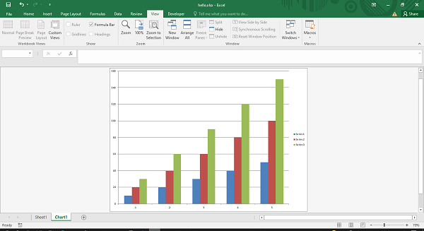
The following code writes the data series in the worksheet names sheet1 but opens a new chartsheet to add a column chart based on the data in sheet1.
import xlsxwriter

wb = xlsxwriter.Workbook('hello.xlsx')
worksheet = wb.add_worksheet()

cs = wb.add_chartsheet()
chart = wb.add_chart({'type': 'column'})

data = [
   [10, 20, 30, 40, 50],
   [20, 40, 60, 80, 100],
   [30, 60, 90, 120, 150],
]
worksheet.write_column('A1', data[0])
worksheet.write_column('B1', data[1])
worksheet.write_column('C1', data[2])

chart.add_series({'values': '=Sheet1!$A$1:$A$5'})
chart.add_series({'values': '=Sheet1!$B$1:$B$5'})
chart.add_series({'values': '=Sheet1!$C$1:$C$5'})

cs.set_chart(chart)
cs.activate()

wb.close()
Output
Exception Class
XlsxWriter identifies various run-time errors or exceptions which can be trapped using Python's error handling technique so as to avoid corruption of Excel files. The Exception classes in XlsxWriter are as follows −
| Sr.No | Exception Classes & Description |
|---|---|
| 1 |
XlsxWriterException Base exception for XlsxWriter. |
| 2 | XlsxFileError Base exception for all file related errors. |
| 3 | XlsxInputError Base exception for all input data related errors. |
| 4 | FileCreateError Occurs if there is a file permission error, or IO error, when writing the xlsx file to disk or if the file is already open in Excel. |
| 5 | UndefinedImageSize Raised with insert_image() method if the image doesn't contain height or width information. The exception is raised during Workbook close(). |
| 6 | UnsupportedImageFormat Raised if the image isn't one of the supported file formats: PNG, JPEG, GIF, BMP, WMF or EMF. |
| 7 | EmptyChartSeries This exception occurs when a chart is added to a worksheet without a data series. |
| 8 | InvalidWorksheetName if a worksheet name is too long or contains invalid characters. |
| 9 | DuplicateWorksheetName This exception is raised when a worksheet name is already present. |
Exception FileCreateError
Assuming that a workbook named hello.xlsx is already opened using Excel app, then the following code will raise a FileCreateError −
import xlsxwriter
workbook = xlsxwriter.Workbook('hello.xlsx')
worksheet = workbook.add_worksheet()
workbook.close()
When this program is run, the error message is displayed as below −
PermissionError: [Errno 13] Permission denied: 'hello.xlsx'
During handling of the above exception, another exception occurred:
Traceback (most recent call last):
   File "hello.py", line 4, in <module>
   workbook.close()
File "e:\xlsxenv\lib\site-packages\xlsxwriter\workbook.py", line 326, in close
   raise FileCreateError(e)
xlsxwriter.exceptions.FileCreateError: [Errno 13] Permission denied: 'hello.xlsx'
Handling the Exception
We can use Python's exception handling mechanism for this purpose.
import xlsxwriter
try:
   workbook = xlsxwriter.Workbook('hello.xlsx')
   worksheet = workbook.add_worksheet()
   workbook.close()
except:
   print ("The file is already open")
Now the custom error message will be displayed.
(xlsxenv) E:\xlsxenv>python ex34.py
The file is already open
Exception EmptyChartSeries
Another situation of an exception being raised when a chart is added with a data series.
import xlsxwriter
workbook = xlsxwriter.Workbook('hello.xlsx')
worksheet = workbook.add_worksheet()
chart = workbook.add_chart({'type': 'column'})
worksheet.insert_chart('A7', chart)
workbook.close()
This leads to EmptyChartSeries exception −
xlsxwriter.exceptions.EmptyChartSeries: Chart1 must contain at least one data series.
Python XlsxWriter - Cell Notation & Ranges
Each worksheet in a workbook is a grid of a large number of cells, each of which can store one piece of data - either value or formula. Each Cell in the grid is identified by its row and column number.
In Excel's standard cell addressing, columns are identified by alphabets, A, B, C, ., Z, AA, AB etc., and rows are numbered starting from 1.
The address of each cell is alphanumeric, where the alphabetic part corresponds to the column and number corresponding to the row. For example, the address "C5" points to the cell in column "C" and row number "5".
Cell Notations
The standard Excel uses alphanumeric sequence of column letter and 1-based row. XlsxWriter supports the standard Excel notation (A1 notation) as well as Row-column notation which uses a zero based index for both row and column.
Example
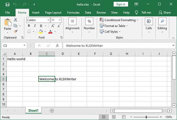
In the following example, a string 'Hello world' is written into A1 cell using Excel's standard cell address, while 'Welcome to XLSXWriter' is written into cell C5 using row-column notation.
import xlsxwriter
wb = xlsxwriter.Workbook('hello.xlsx')
ws = wb.add_worksheet()
ws.write('A1', 'Hello world')           # A1 notation
ws.write(4,2,"Welcome to XLSXWriter")   # Row-column notation
wb.close()
Output
Open the hello.xlsx file using Excel software.
The numbered row-column notation is especially useful when referring to the cells programmatically. In the following code data in a list of lists has to be written to a range of cells in a worksheet. This is achieved by two nested loops, the outer representing the row numbers and the inner loop for column numbers.
data = [
   ['Name', 'Physics', 'Chemistry', 'Maths', 'Total'],
   ['Ravi', 60, 70, 80],
   ['Kiran', 65, 75, 85],
   ['Karishma', 55, 65, 75],
]
for row in range(len(data)):
   for col in range(len(data[row])):
      ws.write(row, col, data[row][col])
The same result can be achieved by using write_row() method of the worksheet object used in the code below −
for row in range(len(data)):
   ws.write_row(6+row,0, data[row])
The worksheet object has add_table() method that writes the data to a range and converts into Excel range, displaying autofilter dropdown arrows in the top row.
ws.add_table('G6:J9', {'data': data, 'header_row':True})
Example
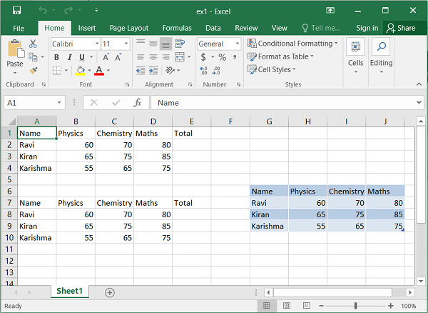
The output of all the three codes above can be verified by the following code and displayed in the following figure −
import xlsxwriter

wb = xlsxwriter.Workbook('ex1.xlsx')
ws = wb.add_worksheet()

data = [
   ['Name', 'Physics', 'Chemistry', 'Maths', 'Total'],
   ['Ravi', 60, 70, 80],
   ['Kiran', 65, 75, 85],
   ['Karishma', 55, 65, 75],
]
for row in range(len(data)):
   for col in range(len(data[row])):
      ws.write(row, col, data[row][col])

for row in range(len(data)):
   ws.write_row(6+row,0, data[row])

ws.add_table('G6:J9', {'data': data, 'header_row':False})

wb.close()
Output
Execute the above program and open the ex1.xlsx using Excel software.
Python XlsxWriter - Defined Names
In Excel, it is possible to identify a cell, a formula, or a range of cells by user-defined name, which can be used as a variable used to make the definition of formula easy to understand. This can be achieved using the define_name() method of the Workbook class.
In the following code snippet, we have a range of cells consisting of numbers. This range has been given a name as marks.
data=['marks',50,60,70, 'Total']
ws.write_row('A1', data)
wb.define_name('marks', '=Sheet1!$A$1:$E$1')
If the name is assigned to a range of cells, the second argument of define_name() method is a string with the name of the sheet followed by "!" symbol and then the range of cells using the absolute addressing scheme. In this case, the range A1:E1 in sheet1 is named as marks.
This name can be used in any formula. For example, we calculate the sum of numbers in the range identified by the name marks.
ws.write('F1', '=sum(marks)')
We can also use the named cell in the write_formula() method. In the following code, this method is used to calculate interest on the amount where the rate is a defined_name.
ws.write('B5', 10)
wb.define_name('rate', '=sheet1!$B$5')

ws.write_row('A5', ['Rate', 10])

data=['Amount',1000, 2000, 3000]
ws.write_column('A6', data)
ws.write('B6', 'Interest')
for row in range(6,9):
   ws.write_formula(row, 1, '= rate*$A{}/100'.format(row+1))
We can also use write_array_formula() method instead of the loop in the above code −
ws.write_array_formula('D7:D9' , '{=rate/100*(A7:A9)}')
Example
The complete code using define_name() method is given below −
import xlsxwriter

wb = xlsxwriter.Workbook('ex2.xlsx')
ws = wb.add_worksheet()

data = ['marks',50,60,70, 'Total']
ws.write_row('A1', data)
wb.define_name('marks', '=Sheet1!$A$1:$E$1')
ws.write('F1', '=sum(marks)')

ws.write('B5', 10)
wb.define_name('rate', '=sheet1!$B$5')

ws.write_row('A5', ['Rate', 10])

data=['Amount',1000, 2000, 3000]
ws.write_column('A6', data)
ws.write('B6', 'Interest')

for row in range(6,9):
   ws.write_formula(row, 1, '= rate*$A{}/100'.format(row+1))

wb.close()
Output
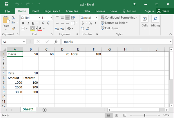
Run the above program and open ex2.xlsx with Excel.
Python XlsxWriter - Formula & Function
The Worksheet class offers three methods for using formulas.
- write_formula()
- write_array_formula()
- write_dynamic_array_formula()
All these methods are used to assign formula as well as function to a cell.
The write_formula() Method
The write_formula() method requires the address of the cell, and a string containing a valid Excel formula. Inside the formula string, only the A1 style address notation is accepted. However, the cell address argument can be either standard Excel type or zero based row and column number notation.
Example
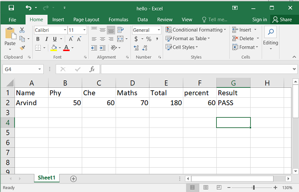
In the example below, various statements use write_formula() method. The first uses a standard Excel notation to assign a formula. The second statement uses row and column number to specify the address of the target cell in which the formula is set. In the third example, the IF() function is assigned to G2 cell.
import xlsxwriter
wb = xlsxwriter.Workbook('hello.xlsx')
ws = wb.add_worksheet()
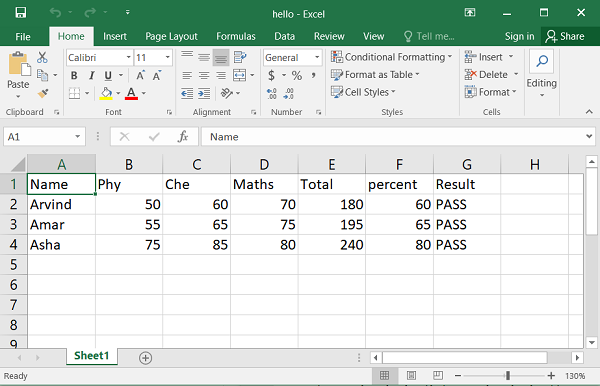
data=[
['Name', 'Phy', 'Che', 'Maths', 'Total', 'percent', 'Result' ],
['Arvind', 50,60,70]
]
ws.write_row('A1', data[0])
ws.write_row('A2', data[1])
ws.write_formula('E2', '=B2+C2+D2')
ws.write_formula(1,5, '=E2*100/300')
ws.write_formula('G2', '=IF(F2>=50, "PASS","FAIL")')
wb.close()
Output
The Excel file shows the following result −
The write_array_formula() Method
The write_array_formula() method is used to extend the formula over a range. In Excel, an array formula performs a calculation on a set of values. It may return a single value or a range of values.
An array formula is indicated by a pair of braces around the formula − {=SUM(A1:B1*A2:B2)}. The range can be either specified by row and column numbers of first and last cell in the range (such as 0,0, 2,2) or by the string representation 'A1:C2'.
Example
In the following example, array formulas are used for columns E, F and G to calculate total, percent and result from marks in the range B2:D4.
import xlsxwriter
wb = xlsxwriter.Workbook('hello.xlsx')
ws = wb.add_worksheet()

data=[
   ['Name', 'Phy', 'Che', 'Maths', 'Total', 'percent', 'Result'],
   ['Arvind', 50,60,70],
   ['Amar', 55,65,75],
   ['Asha', 75,85,80]
]

for row in range(len(data)):
   ws.write_row(row,0, data[row])

ws.write_array_formula('E2:E4', '{=B2:B4+C2:C4+D2:D4}')
ws.write_array_formula(1,5,3,5, '{=(E2:E4)*100/300}')
ws.write_array_formula('G2:G4', '{=IF((F2:F4)>=50, "PASS","FAIL")}')

wb.close()
Output
Here is how the worksheet appears when opened using MS Excel −
The write_dynamic_array_data() Method
The write_dynamic_array_data() method writes an dynamic array formula to a cell range. The concept of dynamic arrays has been introduced in EXCEL's 365 version, and some new functions that leverage the advantage of dynamic arrays have been introduced. These functions are −
| Sr.No | Functions & Description |
|---|---|
| 1 | FILTER Filter data and return matching records |
| 2 | RANDARRAY Generate array of random numbers |
| 3 | SEQUENCE Generate array of sequential numbers |
| 4 | SORT Sort range by column |
| 5 | SORTBY Sort range by another range or array |
| 6 | UNIQUE Extract unique values from a list or range |
| 7 | XLOOKUP replacement for VLOOKUP |
| 8 | XMATCH replacement for the MATCH function |
Dynamic arrays are ranges of return values whose size can change based on the results. For example, a function such as FILTER() returns an array of values that can vary in size depending on the filter results.
Example
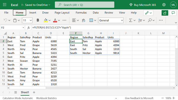
In the example below, the data range is A1:D17. The filter function uses this range and the criteria range is C1:C17, in which the product names are given. The FILTER() function results in a dynamic array as the number of rows satisfying the criteria may change.
import xlsxwriter

wb = xlsxwriter.Workbook('hello.xlsx')
ws = wb.add_worksheet()

data = (
   ['Region', 'SalesRep', 'Product', 'Units'],
   ['East',   'Tom',      'Apple',    6380],
   ['West',   'Fred',     'Grape',    5619],
   ['North',  'Amy',      'Pear',     4565],
   ['South',  'Sal',      'Banana',   5323],
   ['East',   'Fritz',    'Apple',    4394],
   ['West',   'Sravan',   'Grape',    7195],
   ['North',  'Xi',       'Pear',     5231],
   ['South',  'Hector',   'Banana',   2427],
   ['East',   'Tom',      'Banana',   4213],
   ['West',   'Fred',     'Pear',     3239],
   ['North',  'Amy',      'Grape',    6520],
   ['South',  'Sal',      'Apple',    1310],
   ['East',   'Fritz',    'Banana',   6274],
   ['West',   'Sravan',   'Pear',     4894],
   ['North',  'Xi',       'Grape',    7580],
   ['South',  'Hector',   'Apple',    9814])
for row in range(len(data)):
   ws.write_row(row,0, data[row])

ws.write_dynamic_array_formula('F1', '=FILTER(A1:D17,C1:C17="Apple")')
wb.close()
Output
Note that the formula string to write_dynamic_array_formula() need not contain curly brackets. The resultant hello.xlsx must be opened with Excel 365 app.
Python XlsxWriter - Date & Time
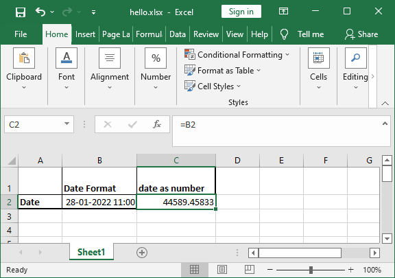
In Excel, dates are stored as real numbers so that they can be used in calculations. By default, January 1, 1900 (called as epoch) is treated 1, and hence January 28, 2022 corresponds to 44589. Similarly, the time is represented as the fractional part of the number, as the percentage of day. Hence, January 28, 2022 11.00 corresponds to 44589.45833.
The set_num_format() Method
Since date or time in Excel is just like any other number, to display the number as a date you must apply an Excel number format to it. Use set_num_format() method of the Format object using appropriate formatting.
The following code snippet displays a number in "dd/mm/yy" format.
num = 44589
format1 = wb.add_format()
format1.set_num_format('dd/mm/yy')
ws.write('B2', num, format1)
The num_format Parameter
Alternatively, the num_format parameter of add_format() method can be set to the desired format.
format1 = wb.add_format({'num_format':'dd/mm/yy'})
ws.write('B2', num, format1)
Example
The following code shows the number in various date formats.
import xlsxwriter

wb = xlsxwriter.Workbook('hello.xlsx')
ws = wb.add_worksheet()

num=44589
ws.write('A1', num)

format2 = wb.add_format({'num_format': 'dd/mm/yy'})
ws.write('A2', num, format2)

format3 = wb.add_format({'num_format': 'mm/dd/yy'})
ws.write('A3', num, format3)

format4 = wb.add_format({'num_format': 'd-m-yyyy'})
ws.write('A4', num, format4)

format5 = wb.add_format({'num_format': 'dd/mm/yy hh:mm'})
ws.write('A5', num, format5)

format6 = wb.add_format({'num_format': 'd mmm yyyy'})
ws.write('A6', num, format6)

format7 = wb.add_format({'num_format': 'mmm d yyyy hh:mm AM/PM'})
ws.write('A7', num, format7)

wb.close()
Output
The worksheet looks like the following in Excel software −

write_datetime() and strptime()
The XlsxWriter's Worksheet object also has write_datetime() method that is useful when handling date and time objects obtained with datetime module of Python's standard library.
The strptime() method returns datetime object from a string parsed according to the given format. Some of the codes used to format the string are given below −
%a |
Abbreviated weekday name |
Sun, Mon |
%A |
Full weekday name |
Sunday, Monday |
%d |
Day of the month as a zero-padded decimal |
01, 02 |
%-d |
day of the month as decimal number |
1, 2.. |
%b |
Abbreviated month name |
Jan, Feb |
%m |
Month as a zero padded decimal number |
01, 02 |
%-m |
Month as a decimal number |
1, 2 |
%B |
Full month name |
January, February |
%y |
Year without century as a zero padded decimal number |
99, 00 |
%-y |
Year without century as a decimal number |
0, 99 |
%Y |
Year with century as a decimal number |
2022, 1999 |
%H |
Hour (24 hour clock) as a zero padded decimal number |
01, 23 |
%-H |
Hour (24 hour clock) as a decimal number |
1, 23 |
%I |
Hour (12 hour clock) as a zero padded decimal number |
01, 12 |
%-I |
Hour (12 hour clock) as a decimal number |
1, 12 |
%p |
locale's AM or PM |
AM, PM |
%M |
Minute as a zero padded decimal number |
01, 59 |
%-M |
Minute as a decimal number |
1, 59 |
%S |
Second as a zero padded decimal number |
01, 59 |
%-S |
Second as a decimal number |
1, 59 |
%c |
locale's appropriate date and time representation |
Mon Sep 30 07:06:05 2022 |
The strptime() method is used as follows −
>>> from datetime import datetime
>>> dt="Thu February 3 2022 11:35:5"
>>> code="%a %B %d %Y %H:%M:%S"
>>> datetime.strptime(dt, code)
datetime.datetime(2022, 2, 3, 11, 35, 5)
This datetime object can now be written into the worksheet with write_datetime() method.
Example
In the following example, the datetime object is written with different formats.
import xlsxwriter
from datetime import datetime
wb = xlsxwriter.Workbook('hello.xlsx')
worksheet = wb.add_worksheet()
dt="Thu February 3 2022 11:35:5"
code="%a %B %d %Y %H:%M:%S"
obj=datetime.strptime(dt, code)
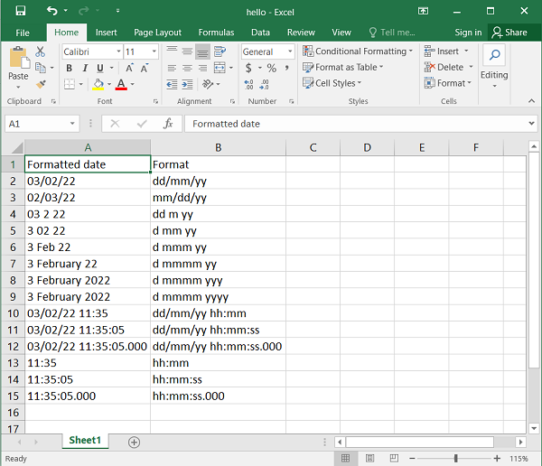
date_formats = (
'dd/mm/yy',
'mm/dd/yy',
'dd m yy',
'd mm yy',
'd mmm yy',
'd mmmm yy',
'd mmmm yyy',
'd mmmm yyyy',
'dd/mm/yy hh:mm',
'dd/mm/yy hh:mm:ss',
'dd/mm/yy hh:mm:ss.000',
'hh:mm',
'hh:mm:ss',
'hh:mm:ss.000',
)
worksheet.write('A1', 'Formatted date')
worksheet.write('B1', 'Format')
row = 1
for fmt in date_formats:
date_format = wb.add_format({'num_format': fmt, 'align': 'left'})
worksheet.write_datetime(row, 0, obj, date_format)
worksheet.write_string(row, 1, fmt)
row += 1
wb.close()
Output
The worksheet appears as follows when opened with Excel.
Python XlsxWriter - Tables
In MS Excel, a Table is a range of cells that has been grouped as a single entity. It can be referenced from formulas and has common formatting attributes. Several features such as column headers, autofilters, total rows, column formulas can be defined in a worksheet table.
The add_table() Method
The worksheet method add_table() is used to add a cell range as a table.
worksheet.add_table(first_row, first_col, last_row, last_col, options)
Both the methods, the standard 'A1' or 'Row/Column' notation are allowed for specifying the range. The add_table() method can take one or more of the following optional parameters. Note that except the range parameter, others are optional. If not given, an empty table is created.
Example
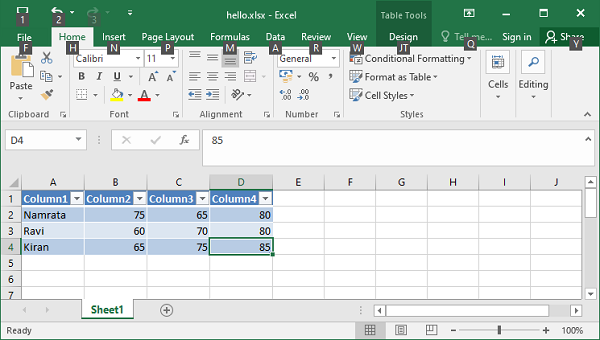
data
This parameter can be used to specify the data in the cells of the table. Look at the following example −
import xlsxwriter
wb = xlsxwriter.Workbook('hello.xlsx')
ws = wb.add_worksheet()

data = [
   ['Namrata',  75, 65, 80],
   ['Ravi',     60, 70, 80],
   ['Kiran',    65, 75, 85],
   ['Karishma', 55, 65, 75],
]
ws.add_table("A1:D4", {'data':data})

wb.close()
Output
Here's the result −
header_row
This parameter can be used to turn on or off the header row in the table. It is on by default. The header row will contain default captions such as Column 1, Column 2, etc. You can set required captions by using the columns parameter.
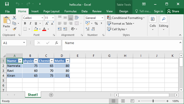
Columns
Example
This property is used to set column captions.
import xlsxwriter

wb = xlsxwriter.Workbook('hello.xlsx')
ws = wb.add_worksheet()

data = [
   ['Namrata',  75, 65, 80],
   ['Ravi',     60, 70, 80],
   ['Kiran',    65, 75, 85],
   ['Karishma', 55, 65, 75],
]

ws.add_table("A1:D4",
{'data':data,
   'columns': [
   {'header': 'Name'},
   {'header': 'physics'},
   {'header': 'Chemistry'},
   {'header': 'Maths'}]
})
wb.close()
Output
The header row is now set as shown −
autofilter
This parameter is ON, by default. When set to OFF, the header row doesn't show the dropdown arrows to set the filter criteria.
Name
In Excel worksheet, the tables are named as Table1, Table2, etc. The name parameter can be used to set the name of the table as required.
ws.add_table("A1:E4", {'data':data, 'name':'marklist'})
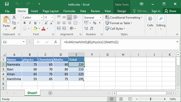
Formula
Column with a formula can be created by specifying formula sub-property in columns options.
Example
In the following example, the table's name property is set to 'marklist'. The formula for 'Total' column E performs sum of marks, and is assigned the value of formula sub-property.
import xlsxwriter

wb = xlsxwriter.Workbook('hello.xlsx')
ws = wb.add_worksheet()

data = [
   ['Namrata',  75, 65, 80],
   ['Ravi',     60, 70, 80],
   ['Kiran',    65, 75, 85],
   ['Karishma', 55, 65, 75],
]
formula = '=SUM(marklist[@[physics]:[Maths]])'
tbl = ws.add_table("A1:E5",
{'data': data,
   'autofilter': False,
   'name': 'marklist',
   'columns': [
      {'header': 'Name'},
      {'header': 'physics'},
      {'header': 'Chemistry'},
      {'header': 'Maths'},
      {'header': 'Total', 'formula': formula}
   ]
})
wb.close()
Output
When the above code is executed, the worksheet shows the Total column with the sum of marks.
Python XlsxWriter - Applying Filter
In Excel, you can set filter on a tabular data based upon criteria using logical expressions. In XlsxWriter's worksheet class, we have autofilter() method or the purpose. The mandatory argument to this method is the cell range. This creates drop-down selectors in the heading row. To apply some criteria, we have two methods available − filter_column() or filter_column_list().
Applying Filter Criteria for a Column
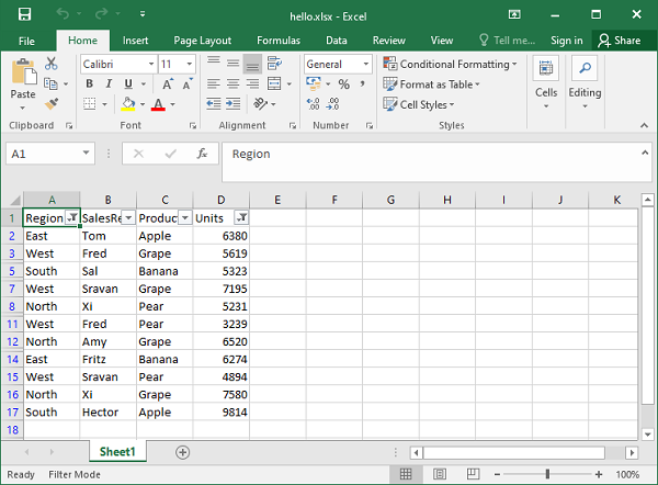
In the following example, the data in the range A1:D51 (i.e. cells 0,0 to 50,3) is used as the range argument for autofilter() method. The filter criteria 'Region == East' is set on 0th column (with Region heading) with filter_column() method.
Example
All the rows in the data range not meeting the filter criteria are hidden by setting hidden option to true for the set_row() method of the worksheet object.
import xlsxwriter

wb = xlsxwriter.Workbook('hello.xlsx')
ws = wb.add_worksheet()

data = (
   ['Region', 'SalesRep', 'Product', 'Units'],
   ['East',   'Tom',      'Apple',    6380],
   ['West',   'Fred',     'Grape',    5619],
   ['North',  'Amy',      'Pear',     4565],
   ['South',  'Sal',      'Banana',   5323],
   ['East',   'Fritz',    'Apple',    4394],
   ['West',   'Sravan',   'Grape',    7195],
   ['North',  'Xi',       'Pear',     5231],
   ['South',  'Hector',   'Banana',   2427],
   ['East',   'Tom',      'Banana',   4213],
   ['West',   'Fred',     'Pear',     3239],
   ['North',  'Amy',      'Grape',    6520],
   ['South',  'Sal',      'Apple',    1310],
   ['East',   'Fritz',    'Banana',   6274],
   ['West',   'Sravan',   'Pear',     4894],
   ['North',  'Xi',       'Grape',    7580],
   ['South',  'Hector',   'Apple',    9814]
)
for row in range(len(data)):
   ws.write_row(row,0, data[row])

ws.autofilter(0, 0, 50, 3)

ws.filter_column(0, 'Region == East')

row = 1
for row_data in (data):
   region = row_data[0]

   if region != 'East':
      ws.set_row(row, options={'hidden': True})

   ws.write_row(row, 0, row_data)

   row += 1
wb.close()
Output
When we open the worksheet with the help of Excel, we will find that only the rows with Region='East' are visible and others are hidden (which you can display again by clearing the filter).
The column parameter can either be a zero indexed column number or a string column name. All the logical operators allowed in Python can be used in criteria (==, !=, , =). Filter criteria can be defined on more than one columns and they can be combined by and or or operators. An example of criteria with logical operator can be as follows −
ws.filter_column('A', 'x > 2000')
ws.filter_column('A', 'x != 2000')
ws.filter_column('A', 'x > 2000 and x
Note that "x" in the criteria argument is just a formal place holder and can be any suitable string as it is ignored anyway internally.
ws.filter_column('A', 'price > 2000')
ws.filter_column('A', 'x != 2000')
ws.filter_column('A', 'marks > 60 and x<75')
XlsxWriter also allows the use of wild cards "*" and "?" in the filter criteria on columns containing string data.
ws.filter_column('A', name=K*') #starts with K
ws.filter_column('A', name=*K*') #contains K
ws.filter_column('A', name=?K*') # second character as K
ws.filter_column('A', name=*K??') #any two characters after K
Example
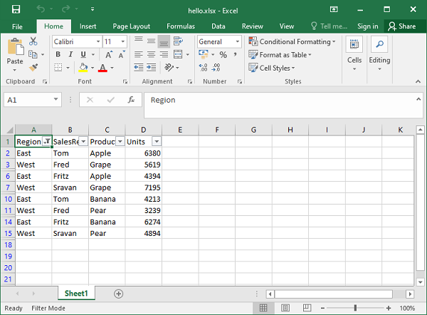
In the following example, first filter on column A requires region to be West and second filter's criteria on column D is "units > 5000". Rows not satisfying the condition "region = West" or "units > 5000" are hidden.
import xlsxwriter
wb = xlsxwriter.Workbook('hello.xlsx')
ws = wb.add_worksheet()
data = (
['Region', 'SalesRep', 'Product', 'Units'],
['East', 'Tom', 'Apple', 6380],
['West', 'Fred', 'Grape', 5619],
['North', 'Amy', 'Pear', 4565],
['South', 'Sal', 'Banana', 5323],
['East', 'Fritz', 'Apple', 4394],
['West', 'Sravan', 'Grape', 7195],
['North', 'Xi', 'Pear', 5231],
['South', 'Hector', 'Banana', 2427],
['East', 'Tom', 'Banana', 4213],
['West', 'Fred', 'Pear', 3239],
['North', 'Amy', 'Grape', 6520],
['South', 'Sal', 'Apple', 1310],
['East', 'Fritz', 'Banana', 6274],
['West', 'Sravan', 'Pear', 4894],
['North', 'Xi', 'Grape', 7580],
['South', 'Hector', 'Apple', 9814])
for row in range(len(data)):
ws.write_row(row,0, data[row])
ws.autofilter(0, 0, 50, 3)
ws.filter_column('A', 'x == West')
ws.filter_column('D', 'x > 5000')
row = 1
for row_data in (data[1:]):
region = row_data[0]
volume = int(row_data[3])
if region == 'West' or volume > 5000:
pass
else:
ws.set_row(row, options={'hidden': True})
ws.write_row(row, 0, row_data)
row += 1
wb.close()
Output
In Excel, the filter icon can be seen on columns A and D headings. The filtered data is seen as below −
Applying a Column List Filter
The filter_column_list() method can be used to represent filters with multiple selected criteria in Excel 2007 style.
ws.filter_column_list(col,list)
The second argument is a list of values against which the data in a given column is matched. For example −
ws.filter_column_list('C', ['March', 'April', 'May'])
It results in filtering the data so that value in column C matches with any item in the list.
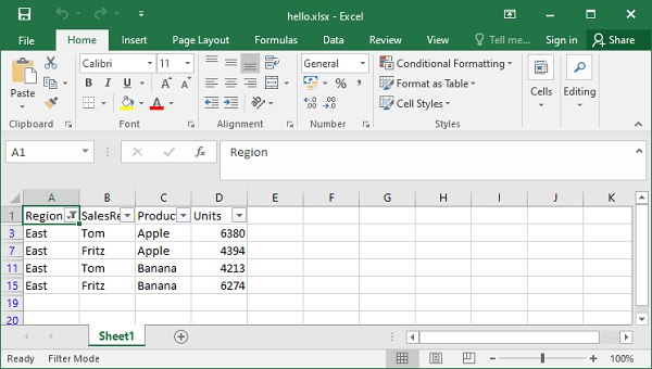
Example
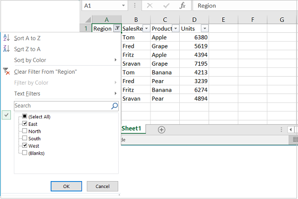
In the following example, the filter_column_list() method is used to filter the rows with region equaling either East or West.
import xlsxwriter
wb = xlsxwriter.Workbook('hello.xlsx')
ws = wb.add_worksheet()
data = (
['Region', 'SalesRep', 'Product', 'Units'],
['East', 'Tom', 'Apple', 6380],
['West', 'Fred', 'Grape', 5619],
['North', 'Amy', 'Pear', 4565],
['South', 'Sal', 'Banana', 5323],
['East', 'Fritz', 'Apple', 4394],
['West', 'Sravan', 'Grape', 7195],
['North', 'Xi', 'Pear', 5231],
['South', 'Hector', 'Banana', 2427],
['East', 'Tom', 'Banana', 4213],
['West', 'Fred', 'Pear', 3239],
['North', 'Amy', 'Grape', 6520],
['South', 'Sal', 'Apple', 1310],
['East', 'Fritz', 'Banana', 6274],
['West', 'Sravan', 'Pear', 4894],
['North', 'Xi', 'Grape', 7580],
['South', 'Hector', 'Apple', 9814]
)
for row in range(len(data)):
ws.write_row(row,0, data[row])
ws.autofilter(0, 0, 50, 3)
l1= ['East', 'West']
ws.filter_column_list('A', l1)
row = 1
for row_data in (data[1:]):
region = row_data[0]
if region not in l1:
ws.set_row(row, options={'hidden': True})
ws.write_row(row, 0, row_data)
row += 1
wb.close()
Output
The Column A shows that the autofilter is applied. All the rows with Region as East or West are displayed and rest are hidden.
From the Excel software, click on the filter selector arrow in the Region heading and we should see that the filter on region equal to East or West is applied.
Python XlsxWriter - Fonts & Colors
Working with Fonts
To perform formatting of worksheet cell, we need to use Format object with the help of add_format() method and configure it with its properties or formatting methods.
f1 = workbook.add_format()
f1 = set_bold(True)
# or
f2 = wb.add_format({'bold':True})
This format object is then used as an argument to worksheet's write() method.
ws.write('B1', 'Hello World', f1)
Example
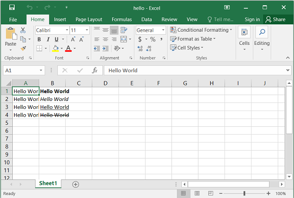
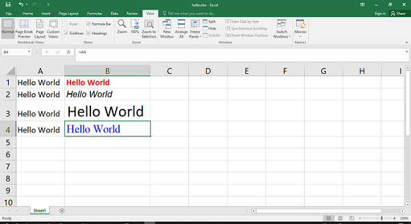
To make the text in a cell bold, underline, italic or strike through, we can either use these properties or corresponding methods. In the following example, the text Hello World is written with set methods.
import xlsxwriter
wb = xlsxwriter.Workbook('hello.xlsx')
ws = wb.add_worksheet()
for row in range(4):
ws.write(row,0, "Hello World")
f1=wb.add_format()
f2=wb.add_format()
f3=wb.add_format()
f4=wb.add_format()
f1.set_bold(True)
ws.write('B1', '=A1', f1)
f2.set_italic(True)
ws.write('B2', '=A2', f2)
f3.set_underline(True)
ws.write('B3', '=A3', f3)
f4.set_font_strikeout(True)
ws.write('B4', '=A4', f4)
wb.close()
Output
Here is the result −
Example
On the other hand, we can use font_color, font_name and font_size properties to format the text as in the following example −
import xlsxwriter
wb = xlsxwriter.Workbook('hello.xlsx')
ws = wb.add_worksheet()
for row in range(4):
ws.write(row,0, "Hello World")
f1=wb.add_format({'bold':True, 'font_color':'red'})
f2=wb.add_format({'italic':True,'font_name':'Arial'})
f3=wb.add_format({'font_size':20})
f4=wb.add_format({'font_color':'blue','font_size':14,'font_name':'Times New Roman'})
ws.write('B1', '=A1', f1)
ws.write('B2', '=A2', f2)
ws.write('B3', '=A3', f3)
ws.write('B4', '=A4', f4)
wb.close()
Output
The output of the above code can be verified by opening the worksheet with Excel −
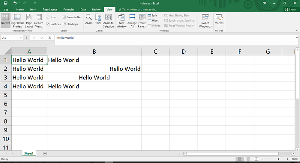
Text Alignment
XlsxWriter's Format object can also be created with alignment methods/properties. The align property can have left, right, center and justify values.
Example
import xlsxwriter
wb = xlsxwriter.Workbook('hello.xlsx')
ws = wb.add_worksheet()
for row in range(4):
ws.write(row,0, "Hello World")
ws.set_column('B:B', 30)
f1=wb.add_format({'align':'left'})
f2=wb.add_format({'align':'right'})
f3=wb.add_format({'align':'center'})
f4=wb.add_format({'align':'justify'})
ws.write('B1', '=A1', f1)
ws.write('B2', '=A2', f2)
ws.write('B3', '=A3', f3)
ws.write('B4', 'Hello World', f4)
wb.close()
Output
The following output shows the text "Hello World" with different alignments. Note that the width of B column is set to 30 by set_column() method of the worksheet object.
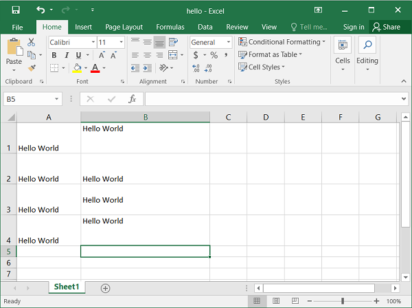
Example
Format object also has valign properties to control vertical placement of the cell.
import xlsxwriter
wb = xlsxwriter.Workbook('hello.xlsx')
ws = wb.add_worksheet()
for row in range(4):
ws.write(row,0, "Hello World")
ws.set_column('B:B', 30)
for row in range(4):
ws.set_row(row, 40)
f1=wb.add_format({'valign':'top'})
f2=wb.add_format({'valign':'bottom'})
f3=wb.add_format({'align':'vcenter'})
f4=wb.add_format({'align':'vjustify'})
ws.write('B1', '=A1', f1)
ws.write('B2', '=A2', f2)
ws.write('B3', '=A3', f3)
ws.write('B4', '=A4', f4)
wb.close()
Output
In the above code, the height of rows 1 to 4 is set to 40 with set_row() method.
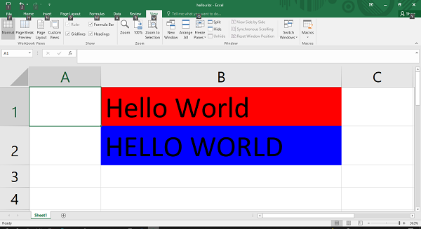
Cell Background and Foreground Colors
Two important properties of Format object are bg_color and fg_color to set the background and foreground color of a cell.
Example
import xlsxwriter
wb = xlsxwriter.Workbook('hello.xlsx')
ws = wb.add_worksheet()
ws.set_column('B:B', 30)
f1=wb.add_format({'bg_color':'red', 'font_size':20})
f2=wb.add_format({'bg_color':'#0000FF', 'font_size':20})
ws.write('B1', 'Hello World', f1)
ws.write('B2', 'HELLO WORLD', f2)
wb.close()
Output
The result of above code looks like this −
Python XlsxWriter - Number Formats
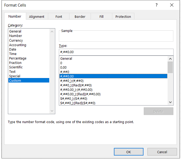
In Excel, different formatting options of numeric data are provided in the Number tab of Format Cells menu.
To control the formatting of numbers with XlsxWriter, we can use the set_num_format() method or define num_format property of add_format() method.
f1 = wb.add_format()
f1.set_num_format(FormatCode)
#or
f1 = wb.add_format('num_format': FormatCode)
Excel has a number of predefined number formats. They can be found under the custom category of Number tab as shown in the above figure. For example, the format code for number with two decimal points and comma separator is #,##0.00.
Example
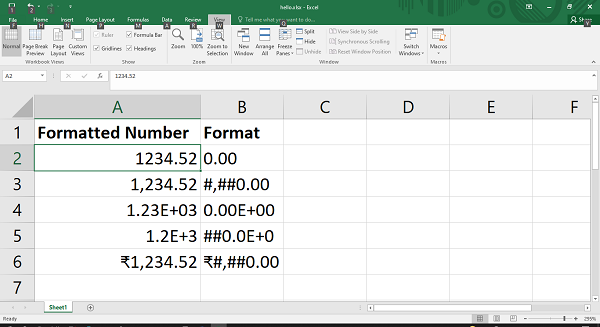
In the following example, a number 1234.52 is formatted with different format codes.
import xlsxwriter
wb = xlsxwriter.Workbook('hello.xlsx')
ws = wb.add_worksheet()
ws.set_column('B:B', 30)
num=1234.52
num_formats = (
'0.00',
'#,##0.00',
'0.00E+00',
'##0.0E+0',
'#,##0.00',
)
ws.write('A1', 'Formatted Number')
ws.write('B1', 'Format')
row = 1
for fmt in num_formats:
format = wb.add_format({'num_format': fmt})
ws.write_number(row, 0, num, format)
ws.write_string(row, 1, fmt)
row += 1
wb.close()
Output
The formatted number along with the format code used is shown in the following figure −
Python XlsxWriter - Border
This section describes how to apply and format the appearance of cell border as well as a border around text box.
Working with Cell Border
The properties in the add_format() method that control the appearance of cell border are as shown in the following table −
Description
Property
method
Cell border
'border'
set_border()
Bottom border
'bottom'
set_bottom()
Top border
'top'
set_top()
Left border
'left'
set_left()
Right border
'right'
set_right()
Border color
'border_color'
set_border_color()
Bottom color
'bottom_color'
set_bottom_color()
Top color
'top_color'
set_top_color()
Left color
'left_color'
set_left_color()
Right color
'right_color'
set_right_color()
Note that for each property of add_format() method, there is a corresponding format class method starting with the set_propertyname() method.
For example, to set a border around a cell, we can use border property in add_format() method as follows −
f1= wb.add_format({ 'border':2})
The same action can also be done by calling the set_border() method −
f1 = workbook.add_format()
f1.set_border(2)
Individual border elements can be configured by the properties or format methods as follows −
- set_bottom()
- set_top()
- set_left()
- set_right()
These border methods/properties have an integer value corresponding to the predefined styles as in the following table −
| Index | Name | Weight | Style |
|---|---|---|---|
| 0 | None | 0 | |
| 1 | Continuous | 1 | ----------- |
| 2 | Continuous | 2 | ----------- |
| 3 | Dash | 1 | - - - - - - |
| 4 | Dot | 1 | . . . . . . |
| 5 | Continuous | 3 | ----------- |
| 6 | Double | 3 | =========== |
| 7 | Continuous | 0 | ----------- |
| 8 | Dash | 2 | - - - - - - |
| 9 | Dash Dot | 1 | - . - . - . |
| 10 | Dash Dot | 2 | - . - . - . |
| 11 | Dash Dot Dot | 1 | - . . - . . |
| 12 | Dash Dot Dot | 2 | - . . - . . |
| 13 | SlantDash Dot | 2 | / - . / - . |
Example
Following code shows how the border property is used. Here, each row is having a border style 2 corresponding to continuous bold.
import xlsxwriter
wb = xlsxwriter.Workbook('hello.xlsx')
ws = wb.add_worksheet()
f1=wb.add_format({'bold':True, 'border':2, 'border_color':'red'})
f2=wb.add_format({'border':2, 'border_color':'red'})
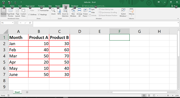
headings = ['Month', 'Product A', 'Product B']
data = [
['Jan', 'Feb', 'Mar', 'Apr', 'May', 'June'],
[10, 40, 50, 20, 10, 50],
[30, 60, 70, 50, 40, 30],
]
ws.write_row('A1', headings, f1)
ws.write_column('A2', data[0], f2)
ws.write_column('B2', data[1],f2)
ws.write_column('C2', data[2],f2)
wb.close()
Output
The worksheet shows a bold border around the cells.
Working with Textbox Border
The border property is also available for the text box object. The text box also has a line property which is similar to border, so that they can be used interchangeably. The border itself can further be formatted by none, color, width and dash_type parameters.
Line or border set to none means that the text box will not have any border. The dash_type parameter can be any of the following values −
- solid
- round_dot
- square_dot
- dash
- dash_dot
- long_dash
- long_dash_dot
- long_dash_dot_dot
Example
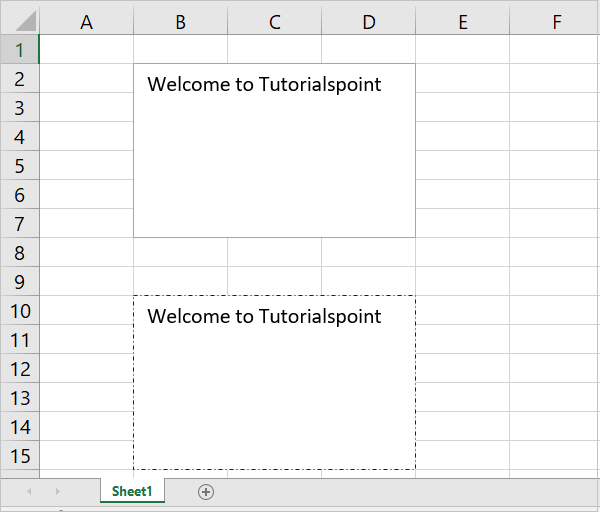
Here is a program that displays two text boxes, one with a solid border, red in color; and the second box has dash_dot type border in blue color.
import xlsxwriter

wb = xlsxwriter.Workbook('hello.xlsx')
ws = wb.add_worksheet()

ws.insert_textbox('B2', 'Welcome to Tutorialspoint',
{'border': {'color': '#FF9900'}})

ws.insert_textbox('B10', 'Welcome to Tutorialspoint', {
   'line':
   {'color': 'blue', 'dash_type': 'dash_dot'}
})
wb.close()
Output
The output worksheet shows the textbox borders.
Python XlsxWriter - Hyperlinks
A hyperlink is a string, which when clicked, takes the user to some other location, such as a URL, another worksheet in the same workbook or another workbook on the computer. Worksheet class provides write_url() method for the purpose. Hyperlinks can also be placed inside a textbox with the use of url property.
First, let us learn about write_url() method. In addition to the Cell location, it needs the URL string to be directed to.
import xlsxwriter

workbook = xlsxwriter.Workbook('hello.xlsx')
worksheet = workbook.add_worksheet()
worksheet.write_url('A1', 'https://www.tutorialspoint.com/index.htm')

workbook.close()
This method has a few optional parameters. One is a Format object to configure the font, color properties of the URL to be displayed. We can also specify a tool tip string and a display text foe the URL. When the text is not given, the URL itself appears in the cell.
Example
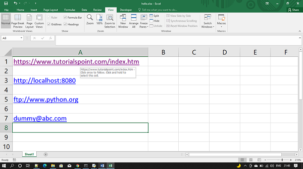
Different types of URLs supported are http://, https://, ftp:// and mailto:. In the example below, we use these URLs.
import xlsxwriter

workbook = xlsxwriter.Workbook('hello.xlsx')
worksheet = workbook.add_worksheet()

worksheet.write_url('A1', 'https://www.tutorialspoint.com/index.htm')
worksheet.write_url('A3', 'http://localhost:8080')
worksheet.write_url('A5', 'ftp://www.python.org')
worksheet.write_url('A7', 'mailto:dummy@abc.com')

workbook.close()
Output
Run the above code and open the hello.xlsx file using Excel.
Example
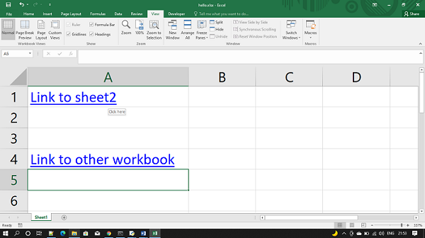
We can also insert hyperlink to either another workskeet in the same workbook, or another workbook. This is done by prefixing with internal: or external: the local URIs.
import xlsxwriter

workbook = xlsxwriter.Workbook('hello.xlsx')
worksheet = workbook.add_worksheet()

worksheet.write_url('A1', 'internal:Sheet2!A1', string="Link to sheet2", tip="Click here")
worksheet.write_url('A4', "external:c:/test/testlink.xlsx", string="Link to other workbook")

workbook.close()
Output
Note that the string and tip parameters are given as an alternative text to the link and tool tip. The output of the above program is as given below −
Python XlsxWriter - Conditional Formatting
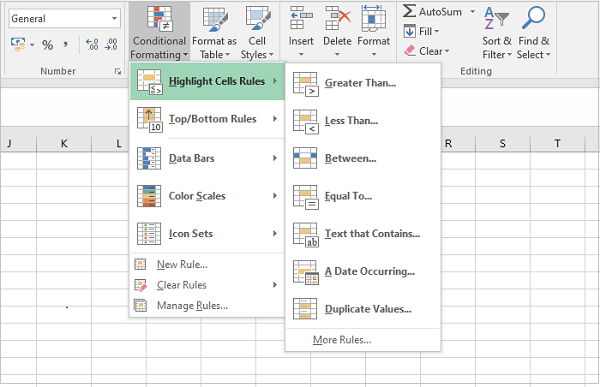
Excel uses conditional formatting to change the appearance of cells in a range based on user defined criteria. From the conditional formatting menu, it is possible to define criteria involving various types of values.
In the worksheet shown below, the column A has different numbers. Numbers less than 50 are shown in red font color and grey background color.
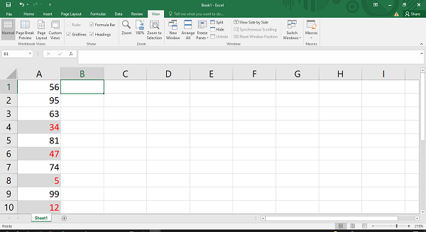
This is achieved by defining a conditional formatting rule below −
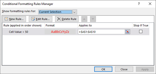
The conditional_format() method
In XlsxWriter, there as a conditional_format() method defined in the Worksheet class. To achieve the above shown result, the conditional_format() method is called as in the following code −
import xlsxwriter

wb = xlsxwriter.Workbook('hello.xlsx')
ws = wb.add_worksheet()

data=[56,95,63,34,81,47,74,5,99,12]
row=0

for num in data:
   ws.write(row,0,num)
   row+=1
f1 = wb.add_format({'bg_color': '#D9D9D9', 'font_color': 'red'})
ws.conditional_format(
   'A1:A10',{
      'type':'cell', 'criteria':'<', 'value':50, 'format':f1
   }
)
wb.close()
Parameters
The conditional_format() method's first argument is the cell range, and the second argument is a dictionary of conditional formatting options.
The options dictionary configures the conditional formatting rules with the following parameters −
The type option is a required parameter. Its value is either cell, date, text, formula, etc. Each parameter has sub-parameters such as criteria, value, format, etc.
Type is the most common conditional formatting type. It is used when a format is applied to a cell based on a simple criterion.
Criteria parameter sets the condition by which the cell data will be evaluated. All the logical operator in addition to between and not between operators are the possible values of criteria parameter.
Value parameter is the operand of the criteria that forms the rule.
Format parameter is the Format object (returned by the add_format() method). This defines the formatting features such as font, color, etc. to be applied to cells satisfying the criteria.
The date type is similar the cell type and uses the same criteria and values. However, the value parameter should be given as a datetime object.
The text type specifies Excel's "Specific Text" style conditional format. It is used to do simple string matching using the criteria and value parameters.
Example
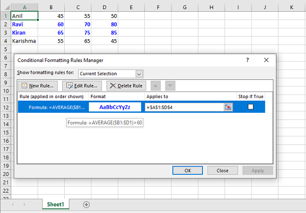
When formula type is used, the conditional formatting depends on a user defined formula.
import xlsxwriter

wb = xlsxwriter.Workbook('hello.xlsx')
ws = wb.add_worksheet()

data = [
   ['Anil', 45, 55, 50], ['Ravi', 60, 70, 80],
   ['Kiran', 65, 75, 85], ['Karishma', 55, 65, 45]
]
for row in range(len(data)):
   ws.write_row(row,0, data[row])

f1 = wb.add_format({'font_color': 'blue', 'bold':True})

ws.conditional_format(
   'A1:D4',
   {
      'type':'formula', 'criteria':'=AVERAGE($B1:$D1)>60', 'value':50, 'format':f1
   })
wb.close()
Output
Open the resultant workbook using MS Excel. We can see the rows satisfying the above condition displayed in blue color according to the format object. The conditional format rule manager also shows the criteria that we have set in the above code.
Python XlsxWriter - Adding Charts
One of the most important features of Excel is its ability to convert data into chart. A chart is a visual representation of data. Different types of charts can be generated from the Chart menu.
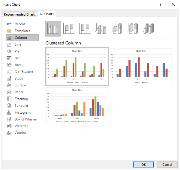
To generate charts programmatically, XlsxWriter library has a Chart class. Its object is obtained by calling add_chart() method of the Workbook class. It is then associated with the data ranges in the worksheet with the help of add_series() method. The chart object is then inserted in the worksheet using its insert_chart() method.
Example
Given below is the code for displaying a simple column chart.
import xlsxwriter
wb = xlsxwriter.Workbook('hello.xlsx')
worksheet = wb.add_worksheet()
chart = wb.add_chart({'type': 'column'})

data = [
   [10, 20, 30,  40,  50],
   [20, 40, 60,  80, 100],
   [30, 60, 90, 120, 150],
]
worksheet.write_column('A1', data[0])
worksheet.write_column('B1', data[1])
worksheet.write_column('C1', data[2])

chart.add_series({'values': '=Sheet1!$A$1:$A$5'})
chart.add_series({'values': '=Sheet1!$B$1:$B$5'})
chart.add_series({'values': '=Sheet1!$C$1:$C$5'})

worksheet.insert_chart('B7', chart)

wb.close()
Output
The generated chart is embedded in the worksheet and appears as follows −

The add_series() method has following additional parameters −
Values − This is the most important property mandatory option. It links the chart with the worksheet data that it displays.
Categories − This sets the chart category labels. If not given, the chart will just assume a sequential series from 1n.
Name − Set the name for the series. The name is displayed in the formula bar.
Line − Set the properties of the series line type such as color and width.
Border − Set the border properties of the series such as color and style.
Fill − Set the solid fill properties of the series such as color.
Pattern − Set the pattern fill properties of the series.
Gradient − Set the gradient fill properties of the series.
data_labels − Set data labels for the series.
Points − Set properties for individual points in a series.
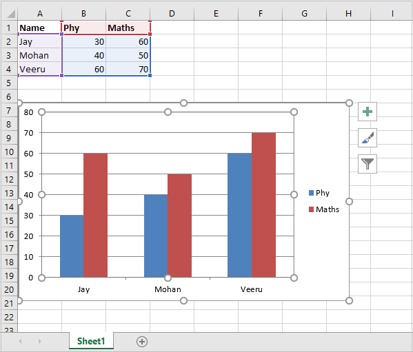
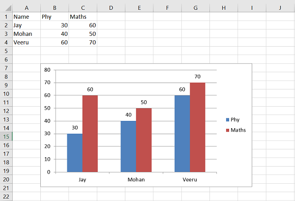
In the following examples, while adding the data series, the value and categories properties are defined. The data for the example is −
# Add the worksheet data that the charts will refer to.
headings = ['Name', 'Phy', 'Maths']
data = [
   ["Jay",   30, 60],
   ["Mohan", 40, 50],
   ["Veeru", 60, 70],
]
After creating the chart object, the first data series corresponds to the column with phy as the value of name property. Names of the students in the first column are used as categories
chart1.add_series({
   'name': '=Sheet1!$B$1',
   'categories': '=Sheet1!$A$2:$A$4',
   'values': '=Sheet1!$B$2:$B$4',
})
The second data series too refers to names in column A as categories and column C with heading as Maths as the values property.
chart1.add_series({
   'name': ['Sheet1', 0, 2],
   'categories': ['Sheet1', 1, 0, 3, 0],
   'values': ['Sheet1', 1, 2, 3, 2],
})
Example
Here is the complete example code −
import xlsxwriter
wb = xlsxwriter.Workbook('hello.xlsx')
worksheet = wb.add_worksheet()
chart1 = wb.add_chart({'type': 'column'})

# Add the worksheet data that the charts will refer to.
headings = ['Name', 'Phy', 'Maths']
data = [
   ["Jay",   30, 60],
   ["Mohan", 40, 50],
   ["Veeru", 60, 70],
]

worksheet.write_row(0,0, headings)
worksheet.write_row(1,0, data[0])
worksheet.write_row(2,0, data[1])
worksheet.write_row(3,0, data[2])

chart1.add_series({
   'name': '=Sheet1!$B$1',
   'categories': '=Sheet1!$A$2:$A$4',
   'values': '=Sheet1!$B$2:$B$4',
})

chart1.add_series({
   'name': ['Sheet1', 0, 2],
   'categories': ['Sheet1', 1, 0, 3, 0],
   'values': ['Sheet1', 1, 2, 3, 2],
})

worksheet.insert_chart('B7', chart1)

wb.close()
Output
The worksheet and the chart based on it appears as follows −
The add_series() method also has data_labels property. If set to True, values of the plotted data points are displayed on top of each column.
Example
Here is the complete code example for add_series() method −
import xlsxwriter
wb = xlsxwriter.Workbook('hello.xlsx')
worksheet = wb.add_worksheet()
chart1 = wb.add_chart({'type': 'column'})

# Add the worksheet data that the charts will refer to.
headings = ['Name', 'Phy', 'Maths']
data = [
   ["Jay",   30, 60],
   ["Mohan", 40, 50],
   ["Veeru", 60, 70],
]

worksheet.write_row(0,0, headings)
worksheet.write_row(1,0, data[0])
worksheet.write_row(2,0, data[1])
worksheet.write_row(3,0, data[2])

chart1.add_series({
   'name': '=Sheet1!$B$1',
   'categories': '=Sheet1!$A$2:$A$4',
   'values': '=Sheet1!$B$2:$B$4',
   'data_labels': {'value':True},
})
chart1.add_series({
   'name': ['Sheet1', 0, 2],
   'categories': ['Sheet1', 1, 0, 3, 0],
   'values': ['Sheet1', 1, 2, 3, 2],
   'data_labels': {'value':True},
})
worksheet.insert_chart('B7', chart1)

wb.close()
Output
Execute the code and open Hello.xlsx. The column chart now shows the data labels.
The data labels can be displayed for all types of charts. Position parameter of data label can be set to top, bottom, left or right.
XlsxWriter supports the following types of charts −
Area − Creates an Area (filled line) style chart.
Bar − Creates a Bar style (transposed histogram) chart.
Column − Creates a column style (histogram) chart.
Line − Creates a Line style chart.
Pie − Creates a Pie style chart.
Doughnut − Creates a Doughnut style chart.
Scatter − Creates a Scatter style chart.
Stock − Creates a Stock style chart.
Radar − Creates a Radar style chart.
Many of the chart types also have subtypes. For example, column, bar, area and line charts have sub types as stacked and percent_stacked. The type and subtype parameters can be given in the add_chart() method.
workbook.add_chart({'type': column, 'subtype': 'stacked'})
The chart is embedded in the worksheet with its insert_chart() method that takes following parameters −
worksheet.insert_chart(location, chartObj, options)
The options parameter is a dictionary that configures the position and scale of chart. The option properties and their default values are −
{
   'x_offset':        0,
   'y_offset':        0,
   'x_scale':         1,
   'y_scale':         1,
   'object_position': 1,
   'description':     None,
   'decorative':      False,
}
The x_offset and y_offset values are in pixels, whereas x_scale and y_scale values are used to scale the chart horizontally / vertically. The description field can be used to specify a description or "alt text" string for the chart.
The decorative parameter is used to mark the chart as decorative, and thus uninformative, for automated screen readers. It has to be set to True/False. Finally, the object_position parameter controls the object positioning of the chart. It allows the following values −
1 − Move and size with cells (the default).
2 − Move but don't size with cells.
3 − Don't move or size with cells.
Python XlsxWriter - Chart Formatting
The default appearance of chart can be customized to make it more appealing, explanatory and user friendly. With XlsxWriter, we can do following enhancements to a Chart object −
Set and format chart title
Set the X and Y axis titles and other parameters
Configure the chart legends
Chat layout options
Setting borders and patterns
Title
You can set and configure the main title of a chart object by calling its set_title() method. Various parameters that can be are as follows −
Name − Set the name (title) for the chart to be displayed above the chart. The name property is optional. The default is to have no chart title.
name_font − Set the font properties for the chart title.
Overlay − Allow the title to be overlaid on the chart.
Layout − Set the (x, y) position of the title in chart relative units.
None − Excel adds an automatic chart title. The none option turns this default title off. It also turns off all other set_title() options.
X and Y axis
The two methods set_x_axis() and set_y_axis() are used to axis titles, the name_font to be used for the title text, the num_font to be used for numbers displayed on the X and Y axis.
name − Set the title or caption for the axis.
name_font − Set the font properties for the axis title.
num_font − Set the font properties for the axis numbers.
num_format − Set the number format for the axis.
major_gridlines − Configure the major gridlines for the axis.
display_units − Set the display units for the axis.
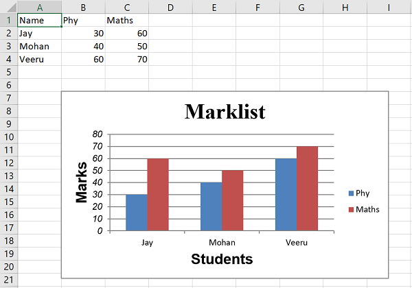
In the previous example, where the data of marklist has been shown in the form of a column chart, we set up the chart formatting options such as the chart title and X as well as Y axis captions and their other display properties as follows −
chart1.set_x_axis(
   {'name': 'Students', 'name_font':{'name':'Arial', 'size':16, 'bold':True},})
chart1.set_y_axis(
   {
      'name': 'Marks', 'name_font':
      {'name':'Arial', 'size':16, 'bold':True}, 'num_font':{'name':'Arial', 'italic':True}
   }
)
Example
Add the above snippet in the complete code. It now looks as given below −
import xlsxwriter

wb = xlsxwriter.Workbook('hello.xlsx')
worksheet = wb.add_worksheet()
chart1 = wb.add_chart({'type': 'column'})

# Add the worksheet data that the charts will refer to.
headings = ['Name', 'Phy', 'Maths']

data = [
   ["Jay", 30, 60],
   ["Mohan", 40, 50],
   ["Veeru", 60, 70],
]

worksheet.write_row(0,0, headings)
worksheet.write_row(1,0, data[0])
worksheet.write_row(2,0, data[1])
worksheet.write_row(3,0, data[2])

chart1.add_series({
   'name': '=Sheet1!$B$1',
   'categories': '=Sheet1!$A$2:$A$4',
   'values': '=Sheet1!$B$2:$B$4',
})

chart1.add_series({
   'name': ['Sheet1', 0, 2],
   'categories': ['Sheet1', 1, 0, 3, 0],
   'values': ['Sheet1', 1, 2, 3, 2],
})
chart1.set_title ({'name': 'Marklist',
   'name_font': {'name':'Times New Roman', 'size':24}
})
chart1.set_x_axis({'name': 'Students',
   'name_font': {'name':'Arial', 'size':16, 'bold':True},
})
chart1.set_y_axis({'name': 'Marks',
   'name_font':{'name':'Arial', 'size':16, 'bold':True},
   'num_font':{'name':'Arial', 'italic':True}
})
worksheet.insert_chart('B7', chart1)

wb.close()
Output
The chart shows the title and axes captions as follows −
Python XlsxWriter - Chart Legends
Depending upon the type of chart, the data is visually represented in the form of columns, bars, lines, arcs, etc. in different colors or patterns. The chart legend makes it easy to quickly understand which color/pattern corresponds to which data series.
Working with Chart Legends
To set the legend and configure its properties such as position and font, XlsxWriter has set_legend() method. The properties are −
None − In Excel chart legends are on by default. The none=True option turns off the chart legend.
Position − Set the position of the chart legend. It can be set to top, bottom, left, right, none.
Font − Set the font properties (like name, size, bold, italic etc.) of the chart legend.
Border − Set the border properties of the legend such as color and style.
Fill − Set the solid fill properties of the legend such as color.
Pattern − Set the pattern fill properties of the legend.
Gradient − Set the gradient fill properties of the legend.
Some of the legend properties are set for the chart as below −
chart1.set_legend(
   {'position':'bottom', 'font': {'name':'calibri','size': 9, 'bold': True}}
)
Example
Here is the complete code to display legends as per the above characteristics −
import xlsxwriter

wb = xlsxwriter.Workbook('hello.xlsx')
worksheet = wb.add_worksheet()
chart1 = wb.add_chart({'type': 'column'})

# Add the worksheet data that the charts will refer to.
headings = ['Name', 'Phy', 'Maths']
data = [
   ["Jay", 30, 60],
   ["Mohan", 40, 50],
   ["Veeru", 60, 70],
]

worksheet.write_row(0,0, headings)
worksheet.write_row(1,0, data[0])
worksheet.write_row(2,0, data[1])
worksheet.write_row(3,0, data[2])
chart1.add_series({
   'name': '=Sheet1!$B$1',
   'categories': '=Sheet1!$A$2:$A$4',
   'values': '=Sheet1!$B$2:$B$4',
})
chart1.add_series({
   'name': ['Sheet1', 0, 2],
   'categories': ['Sheet1', 1, 0, 3, 0],
   'values': ['Sheet1', 1, 2, 3, 2],
})
chart1.set_title ({'name': 'Marklist', 'name_font':
   {'name':'Times New Roman', 'size':24}})

chart1.set_x_axis({'name': 'Students', 'name_font':
   {'name':'Arial', 'size':16, 'bold':True},})

chart1.set_y_axis({'name': 'Marks','name_font':
   {'name':'Arial', 'size':16, 'bold':True},
   'num_font':{'name':'Arial', 'italic':True}})

chart1.set_legend({'position':'bottom', 'font':
   {'name':'calibri','size': 9, 'bold': True}})

worksheet.insert_chart('B7', chart1)

wb.close()
Output
The chart shows the legend below the caption of the X axis.
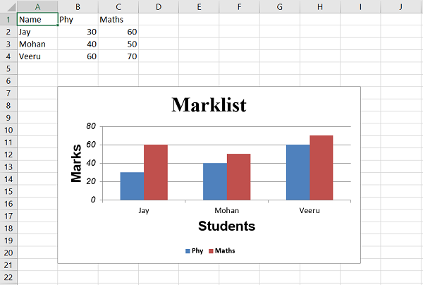
In the chart, the columns corresponding to physics and maths are shown in different colors. The small colored box symbols to the right of the chart are the legends that show which color corresponds to physics or maths.
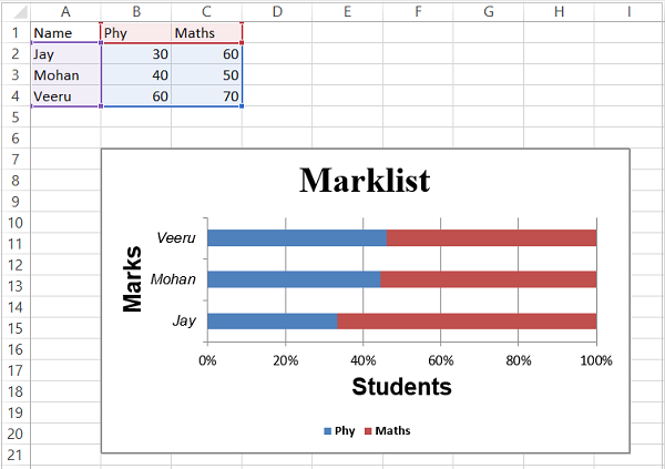
Python XlsxWriter - Bar Chart
The bar chart is similar to a column chart, except for the fact that the data is represented in proportionate horizontal bars instead of vertical columns. To produce a bar chart, the type argument of add_chart() method must be set to 'bar'.
chart1 = workbook.add_chart({'type': 'bar'})
The bar chart appears as follows −
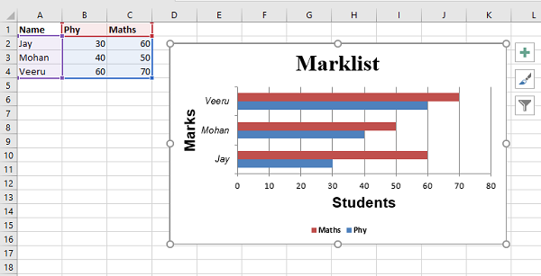
There are two subtypes of bar chart, namely stacked and percent_stacked. In the stacked chart, the bars of different colors for a certain category are placed one after the other. In a percent_stacked chart, the length of each bar shows its percentage in the total value in each category.
chart1 = workbook.add_chart({
   'type': 'bar',
   'subtype': 'percent_stacked'
})
Example
Program to generate percent stacked bar chart is given below −
import xlsxwriter

wb = xlsxwriter.Workbook('hello.xlsx')
worksheet = wb.add_worksheet()
chart1 = wb.add_chart({'type': 'bar', 'subtype': 'percent_stacked'})

# Add the worksheet data that the charts will refer to.
headings = ['Name', 'Phy', 'Maths']
data = [
   ["Jay", 30, 60],
   ["Mohan", 40, 50],
   ["Veeru", 60, 70],
]

worksheet.write_row(0,0, headings)
worksheet.write_row(1,0, data[0])
worksheet.write_row(2,0, data[1])
worksheet.write_row(3,0, data[2])

chart1.add_series({
   'name': '=Sheet1!$B$1',
   'categories': '=Sheet1!$A$2:$A$4',
   'values': '=Sheet1!$B$2:$B$4',
})

chart1.add_series({
   'name': ['Sheet1', 0, 2],
   'categories': ['Sheet1', 1, 0, 3, 0],
   'values': ['Sheet1', 1, 2, 3, 2],
})
chart1.set_title ({'name': 'Marklist', 'name_font':
   {'name':'Times New Roman', 'size':24}})

chart1.set_x_axis({'name': 'Students', 'name_font':
   {'name':'Arial', 'size':16, 'bold':True}, })

chart1.set_y_axis({'name': 'Marks','name_font':
   {'name':'Arial', 'size':16, 'bold':True},
   'num_font':{'name':'Arial', 'italic':True}})

chart1.set_legend({'position':'bottom', 'font':
   {'name':'calibri','size': 9, 'bold': True}})

worksheet.insert_chart('B7', chart1)

wb.close()
Output
The output file will look like the one given below −
Python XlsxWriter - Line Chart
A line shows a series of data points connected with a line along the X-axis. It is an independent axis because the values on the X-axis do not depend on the vertical Y-axis.
The Y-axis is a dependent axis because its values depend on the X-axis and the result is the line that progress horizontally.
Working with XlsxWriter Line Chart
To generate the line chart programmatically using XlsxWriter, we use add_series(). The type of chart object is defined as 'line'.
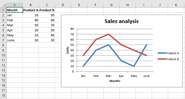
Example
In the following example, we shall plot line chart showing the sales figures of two products over six months. Two data series corresponding to sales figures of Product A and Product B are added to the chart with add_series() method.
import xlsxwriter

wb = xlsxwriter.Workbook('hello.xlsx')
worksheet = wb.add_worksheet()
headings = ['Month', 'Product A', 'Product B']

data = [
   ['Jan', 'Feb', 'Mar', 'Apr', 'May', 'June'],
   [10, 40, 50, 20, 10, 50],
   [30, 60, 70, 50, 40, 30],
]

bold=wb.add_format({'bold':True})
worksheet.write_row('A1', headings, bold)
worksheet.write_column('A2', data[0])
worksheet.write_column('B2', data[1])
worksheet.write_column('C2', data[2])

chart1 = wb.add_chart({'type': 'line'})

chart1.add_series({
   'name': '=Sheet1!$B$1',
   'categories': '=Sheet1!$A$2:$A$7',
   'values': '=Sheet1!$B$2:$B$7',
})
chart1.add_series({
   'name': ['Sheet1', 0, 2],
   'categories': ['Sheet1', 1, 0, 6, 0],
   'values': ['Sheet1', 1, 2, 6, 2],
})
chart1.set_title ({'name': 'Sales analysis'})
chart1.set_x_axis({'name': 'Months'})
chart1.set_y_axis({'name': 'Units'})

worksheet.insert_chart('D2', chart1)

wb.close()
Output
After executing the above program, here is how XlsxWriter generates the Line chart −
Along with data_labels, the add_series() method also has a marker property. This is especially useful in a line chart. The data points are indicated by marker symbols such as a circle, triangle, square, diamond etc. Let us assign circle and square symbols to the two data series in this chart.
chart1.add_series({
   'name': '=Sheet1!$B$1',
   'categories': '=Sheet1!$A$2:$A$7',
   'values': '=Sheet1!$B$2:$B$7',
   'data_labels': {'value': True},
   'marker': {'type': 'circle'},
})
chart1.add_series({
   'name': ['Sheet1', 0, 2],
   'categories': ['Sheet1', 1, 0, 6, 0],
   'values': ['Sheet1', 1, 2, 6, 2],
   'data_labels': {'value': True},
   'marker': {'type': 'square'},})
The data labels and markers are added to the line chart.
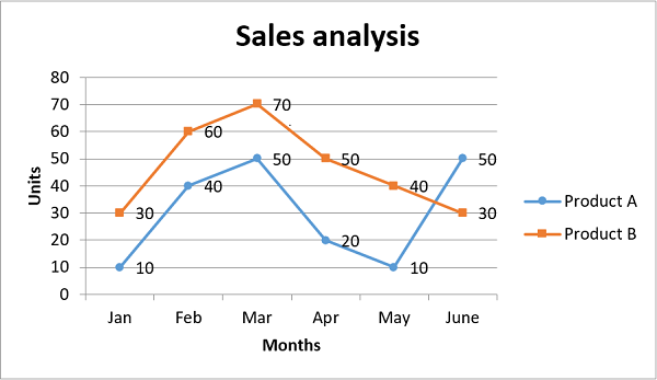
Line chart also supports stacked and percent_stacked subtypes.
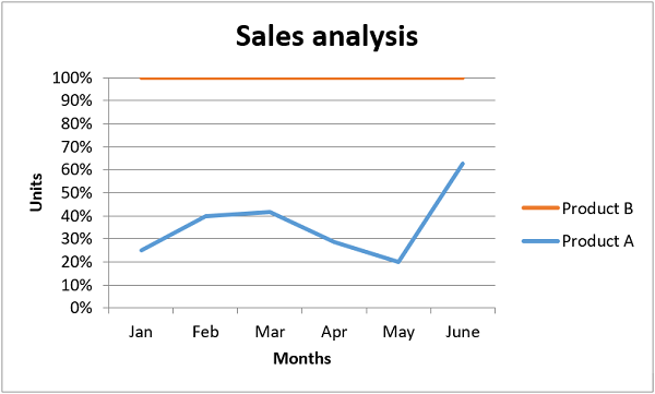
Python XlsxWriter - Pie Chart
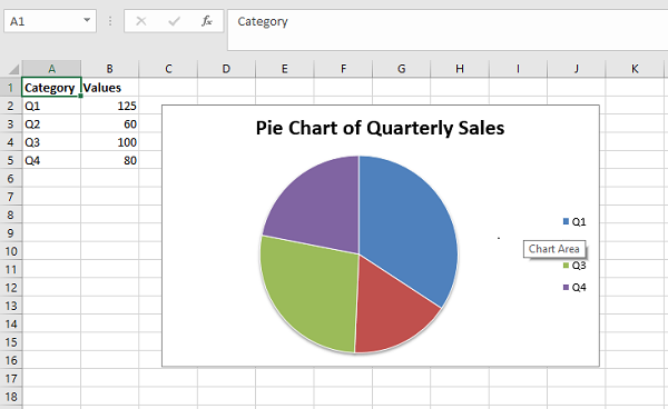
A pie chart is a representation of a single data series into a circle, which is divided into slices corresponding to each data item in the series. In a pie chart, the arc length of each slice is proportional to the quantity it represents. In the following worksheet, quarterly sales figures of a product are displayed in the form of a pie chart.
Working with XlsxWriter Pie Chart
To generate the above chart programmatically using XlsxWriter, we first write the following data in the worksheet.
headings = ['Category', 'Values']
data = [
   ['Q1', 'Q2', 'Q3', 'Q4'],
   [125, 60, 100, 80],
]
worksheet.write_row('A1', headings, bold)
worksheet.write_column('A2', data[0])
worksheet.write_column('B2', data[1])
A Chart object with type=pie is declared and the cell range B1:D1 is used as value parameter for add_series() method and the quarters (Q1, Q2, Q3 and Q4) in column A are the categories.
chart1.add_series({
   'name': 'Quarterly sales data',
   'categories': ['Sheet1', 1, 0, 4, 0],
   'values': ['Sheet1', 1, 1, 4, 1],
})
chart1.set_title({'name': 'Pie Chart of Quarterly Sales'})
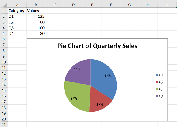
In the pie chart, we can use data_labels property to represent the percent value of each pie by setting percentage=True.
Example
The complete program for pie chart generation is as follows −
import xlsxwriter

wb = xlsxwriter.Workbook('hello.xlsx')
worksheet = wb.add_worksheet()

headings = ['Category', 'Values']
data = [
   ['Q1', 'Q2', 'Q3', 'Q4'],
   [125, 60, 100, 80],
]
bold=wb.add_format({'bold':True})
worksheet.write_row('A1', headings, bold)
worksheet.write_column('A2', data[0])
worksheet.write_column('B2', data[1])

chart1 = wb.add_chart({'type': 'pie'})
chart1.add_series({
   'name': 'Quarterly sales data',
   'categories': ['Sheet1', 1, 0, 4, 0],
   'values': ['Sheet1', 1, 1, 4, 1],
   'data_labels': {'percentage':True},
})
chart1.set_title({'name': 'Pie Chart of Quarterly Sales'})

worksheet.insert_chart('D2', chart1)

wb.close()
Output
Have a look at the pie chart that the above program produces.
Doughnut Chart
The doughnut chart is a variant of the pie chart, with a hole in its center, and it displays categories as arcs rather than slices. Both make part-to-whole relationships easy to grasp at a glance. Just change the chart type to doughnut.
chart1 = workbook.add_chart({'type': 'doughnut'})
The doughnut chart of the data in above example appears as below −
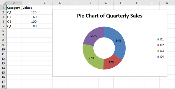
Python XlsxWriter - Sparklines
A sparkline is a small chart, that doesn't have axes or coordinates. It gives a representation of variation of a certain parameter. Normal charts are bigger in size, with a lot of explanatory features such as title, legend, data labels etc. and are set off from the accompanying text. Sparkline on the other hand is small in size and can be embedded inside the text, or a worksheet cell that has its context.
Feature of Sparkline was introduced by Edward Tufte in 1983. Microsoft introduced sparklines in Excel 2010. We can find sparkline option in the insert ribbon of Excel software.
Sparklines are of three types −
line − Similar to line chart
column − Similar to column chart
win_loss − Whether each value is positive (win) or negative (loss).
Working with XlsxWriter Sparklines
XlsxWriter module has add_sparkline() method. It basically needs the cell location of the sparkline and the data range to be represented as a sparkline. Optionally, other parameters such as type, style, etc. are provided in the form of dictionary object. By default, the type is line.
Example
Following program represents same list of numbers in line and column sparklines.
import xlsxwriter

wb = xlsxwriter.Workbook('hello.xlsx')
ws = wb.add_worksheet()

data=[12,23,9,17,31,3,7,21,10,15]

ws.write_row('A1', data)
ws.set_column('K:K', 40)
ws.set_row(0, 30)
ws.add_sparkline('K1', {'range':'Sheet1!A1:J1'})

ws.write_row('A5', data)
ws.set_column('K:K', 40)
ws.set_row(4, 30)
ws.add_sparkline('K5', {'range':'Sheet1!A5:J5', 'type':'column'})

wb.close()
Output
In cell K, the sparklines are added.
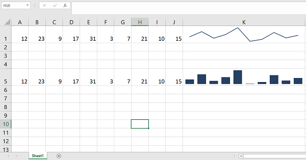
The properties are −
range − is the mandatory parameter. It specifies the cell data range that the sparkline will plot.
type − specifies the type of sparkline. There are 3 available sparkline types are line, column and win_loss.
markers − Turn on the markers for line style sparklines
style − The sparkline styles defined in MS Excel. There are 36 style types.
negative_points − If set to True, the negative points in a sparkline are highlighted.
Example
The following program produces a line sparkline with markers and a win_loss sparkline having negative points highlighted.
import xlsxwriter

wb = xlsxwriter.Workbook('hello.xlsx')
ws = wb.add_worksheet()

data=[12,23,9,17,31,3,7,21,10,15]
ws.write_row('A1', data)
ws.set_column('K:K', 40)
ws.set_row(0, 30)

data=[1,1,-1,-1,-1,1,1,1,-1,-1]
ws.write_row('A5', data)
ws.set_column('K:K', 40)
ws.set_row(4, 30)
ws.add_sparkline('K1', {'range':'Sheet1!A1:J1', 'markers':True})
ws.add_sparkline('K5', {'range':'Sheet1!A5:J5', 'type':'win_loss',
'negative_points':True})

wb.close()
Output
Line Sparkline in K1 has markers. The sparkline in K5 shows negative points highlighting.
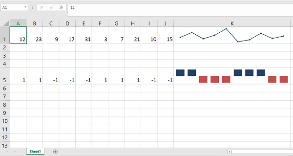
Example Style Types
Following code displays a series of numbers in column sparkline. Ten different style types are used here.
import xlsxwriter

wb = xlsxwriter.Workbook('hello.xlsx')
ws = wb.add_worksheet()

data=[12,23,9,17,31,3,7,21,10,15]
ws.write_row('C3', data)
ws.set_column('B:B',40)

for i in range(1,11):
   ws.write(i+4,0, 'style {}'.format(i))
   ws.add_sparkline(i+4,1,
   {'range':'Sheet1!$C$3:$L$3',
   'type':'column',
   'style':i})

wb.close()
Output
It will produce the following output −
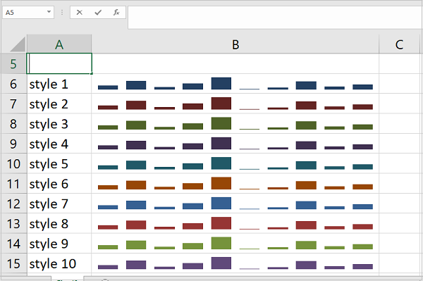
Python XlsxWriter - Data Validation
Data validation feature in Excel allows you to control what a user can enter into a cell. You can use it to ensure that the value in a cell is a number/date within a specified range, text with required length, or to present a dropdown menu to choose the value from.
The data validation tools are available in the Data menu. The first tab allows you to set a validation criterion. Following figure shows that criteria requires the cell should contain an integer between 1 to 25 −
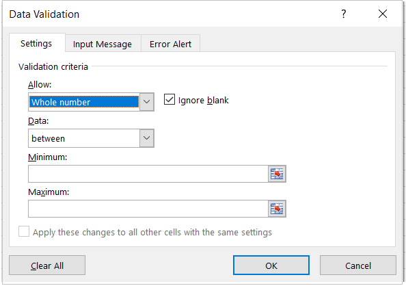
In the second tab, set the message to be flashed when user's cursor is on the desired cell, which in this case is 'Enter any integer between 1 to 25'. You can also set the message title; in this case it is Age.
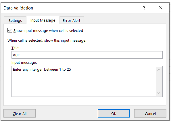
The third tab allows asks you to define any error message you would like to flash if the validation criteria fails.
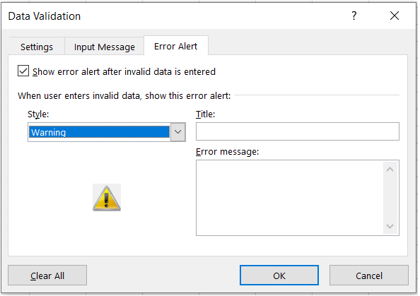
When the user places the cursor in I10 (for which the validation is set), you can see the input message.
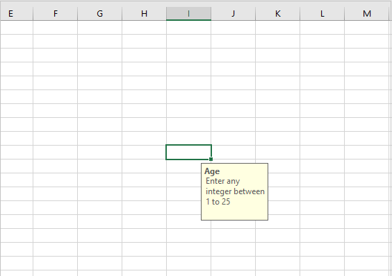
When the entered number is not in the range, the error message will flash.
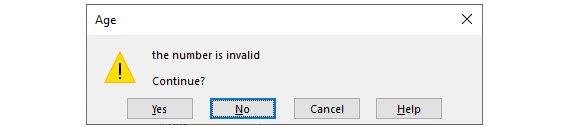
Working with XlsxWriter Data Validation
You can set the validation criteria, input and error message programmatically with data_validation() method.
worksheet.data_validation(
   'I10',
   {
      'validate': 'integer','criteria': 'between',
      'minimum': 1,'maximum': 25,
      'input_title': 'Enter an integer:',
      'input_message': 'between 1 and 25',
      'error_title': 'Input value is not valid!',
      'error_message': 'It  should be an integer between 1 and 25'
   }
)
The data_validation() method accepts options parameter as a dictionary with following parameters −
validate − It is used to set the type of data that you wish to validate. Allowed values are integer, decimal, list, date, time, length etc.
criteria − It is used to set the criteria for validation. It can be set to any logical operator including between/ not between, ==, !=, <, >, <=, >=, etc.
value − Sets the limiting value to which the criteria is applied. It is always required. When using the list validation, it is given as a Comma Separated Variable string.
input_title − Used to set the title of the input message when the cursor is placed in the target cell.
input_message − The message to be displayed when a cell is entered.
error_title − The title of the error message to be displayed when validation criteria is not met.
error_message − Sets the error message. The default error message is "The value you entered is not valid. A user has restricted values that can be entered into the cell."
Example
Following usage of data_validation() method results in the behavior of data validation feature as shown in the above figures.
import xlsxwriter

wb = xlsxwriter.Workbook('hello.xlsx')
worksheet = wb.add_worksheet()

worksheet.data_validation(
   'I10',
   {
      'validate': 'integer','criteria': 'between',
      'minimum': 1,'maximum': 25,
      'input_title': 'Enter an integer:',
      'input_message': 'between 1 and 25',
      'error_title': 'Input value is not valid!',
      'error_message':'It should be an integer between 1 and 25'
   }
)
wb.close()
As another example, the cell I10 is set a validation criterion so as to force the user choose its value from a list of strings in a drop down.
worksheet.data_validation(
   'I10',
   {
      'validate': 'list',
      'source': ['Mumbai', 'Delhi', 'Chennai', 'Kolkata'],
      'input_title': 'Choose one:',
      'input_message': 'Select a value from th list',
   }
)
Example
The modified program for validation with the drop down list is as follows −
import xlsxwriter

wb = xlsxwriter.Workbook('hello.xlsx')
worksheet = wb.add_worksheet()

worksheet.data_validation(
   'I10',
   {
      'validate': 'list',
      'source': ['Mumbai', 'Delhi', 'Chennai', 'Kolkata'],
      'input_title': 'Choose one:',
      'input_message': 'Select a value from the list',
   }
)
wb.close()
Output
The dropdown list appears when the cursor is placed in I10 cell −
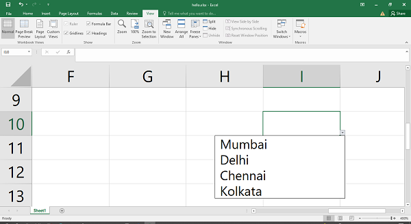
Example
If you want to make the user enter a string of length greater than 5, use >= as criteria and value set to 5.
import xlsxwriter

wb = xlsxwriter.Workbook('hello.xlsx')
worksheet = wb.add_worksheet()

worksheet.data_validation(
   'I10',{
      'validate': 'length',
      'criteria': '>=','value': 5,'input_title': 'Enter name:',
      'input_message': 'Minimum length 5 character',
      'error_message':'Name should have at least 5 characters'
   }
)

wb.close()
Output
If the string is having less than 5 characters, the error message pops up as follows −
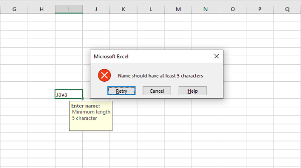
Python XlsxWriter - Outlines & Grouping
In Excel, you can group rows or columns having same value of a particular column (or row)) so that they can be hidden or displayed with a single mouse click. This feature is called to as outlines and grouping. It helps in displaying sub-totals or summaries. This feature can be found in MS excel software's Data→Outline group.
To use this feature, the data range must have all rows should be in the sorted order of values in one column. Suppose we have sales figures of different items. After sorting the range on name of item, click on the Subtotal option in the Outline group. Following dialog box pops up.
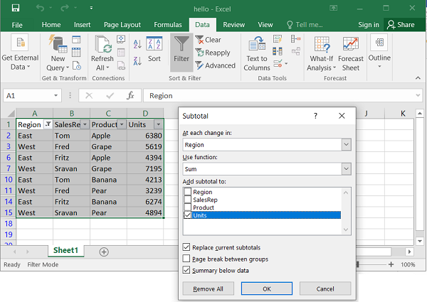
The worksheet shows item-wise subtotal of sales and at the end the grand total. On the left of the worksheet, the outline levels are shown. The original data is at level 3, the subtotals at level 2 and grand total at level 1.
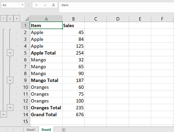
Working with Outlines and Grouping
To do this using XlsxWriter, we need to use the level property of the set_row() method. The data rows are set at level 2.
ws.set_row(row, None, None, {'level': 2})
The rows for subtotal are having level 1.
ws.set_row(row, None, None, {'level': 1})
We use SUBTOTAL() function to calculate and display the sum of sales figures in one group.
Example
The complete code is given below −
import xlsxwriter
wb = xlsxwriter.Workbook('hello.xlsx')
ws = wb.add_worksheet()

headings=['Item', 'Sales']
data=[
   ['Apple', 45], ['Apple', 84], ['Apple', 125],
   ['Mango', 32], ['Mango', 65], ['Mango', 90],
   ['Oranges', 60], ['Oranges', 75], ['Oranges',100],
]
ws.write_row('A1', headings)
item='Apple'
rownum=1
startrow=1
for row in data:
   if row[0]==item:
      ws.set_row(rownum, None, None, {'level': 2})
      ws.write_row(rownum,0, row)
      rownum+=1
else:
   ws.set_row(rownum, None, None, {'level': 1})
   ws.write(rownum, 0, item+' Subtotal')
   cellno='B{}:B{}'.format(startrow,rownum)
   print (cellno)
   ws.write(rownum,1,'=SUBTOTAL(9,'+cellno+')')
   # rownum+=1
   item=data[rownum][0]
   rownum+=1
   ws.set_row(rownum, None, None, {'level': 2})
   ws.write_row(rownum,0, row)
   rownum+=1
   startrow=rownum
else:
   ws.set_row(rownum, None, None, {'level': 1})
   ws.write(rownum, 0, item+' Subtotal')
   cellno='B{}:B{}'.format(startrow,rownum)
   ws.write(rownum,1,'=SUBTOTAL(9,'+cellno+')')
rownum+=1
ws.write(rownum, 0, 'Grand Total')
cellno='B{}:B{}'.format(1,rownum)
ws.write(rownum,1,'=SUBTOTAL(9,'+cellno+')')

wb.close()
Output
Run the code and open hello.xlsx using Excel. As we can see, the outlines are displayed on the left.
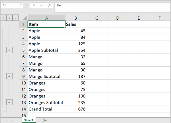
At each level, the minus sign indicates that the rows can be collapsed and only the subtotal row will be displayed.
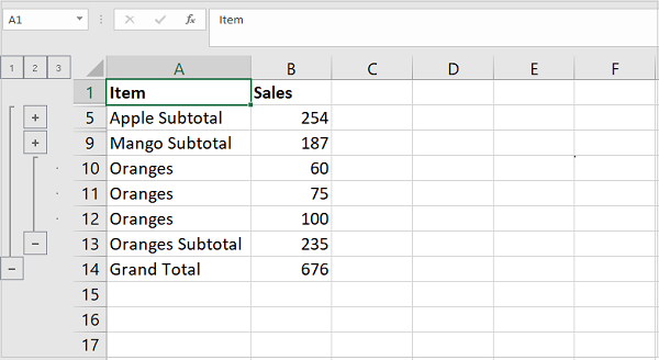
This figure shows all rows at level 2 have been collapsed. It now shows plus symbol in the outline which means that the data rows can be expanded. If you click the minus symbol at level 1, only the grand total will remain on the worksheet.
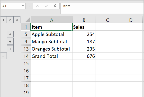
Python XlsxWriter - Freeze & Split Panes
The freeze_panes() method
The freeze_panes() method of Worksheet object in XlsxWriter library divides or splits the worksheet into horizontal or vertical regions known as panes, and "freezes" either or both of these panes so that if we scroll down or scroll down or scroll towards right, the panes (top or left respectively) remains stationary.
The method requires the parameters row and col to specify the location of the split. It should be noted that the split is specified at the top or left of a cell and that the method uses zero based indexing. You can set one of the row and col parameters as zero if you do not want either a vertical or horizontal split.
Example
The worksheet in the following example displays incrementing multiples of the column number in each row, so that each cell displays product of row number and column number.
import xlsxwriter

wb = xlsxwriter.Workbook('hello.xlsx')
worksheet = wb.add_worksheet()
format1=wb.add_format({'bg_color':'#D9D9D9', 'bold':True})

for col in range(0, 15):
   worksheet.write(0, col, col+1, format1)

for row in range(1, 51):
   for col in range(0,15):
      if col==0:
         worksheet.write(row,col,(col+1)*(row + 1), format1)
      else:
         worksheet.write(row,col,(col+1)*(row + 1))
# Freeze pane on the top row.
worksheet.freeze_panes(1, 0)

wb.close()
Output
We then freeze the top row pane. As a result, after opening the worksheet, if the cell pointer is scrolled down, the top row always remains on the worksheet.
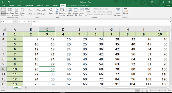
Similarly, we can make the first column stationery.
# Freeze pane on the first column.
worksheet.freeze_panes(0, 1)
The following screenshot shows that column A remains visible even if we scroll towards the right.
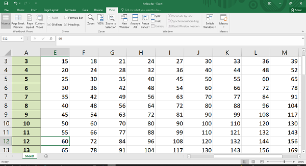
By setting row and column parameter in freeze_panes() method to 1, both the top row and leftmost column will freeze.
# Freeze pane on the first row, first column.
worksheet.freeze_panes(1, 1)
Open the resulting worksheet and scroll the cell cursor around. You will find that row and column numbers in top row and leftmost column, which have been formatted in bold and with a background color, are visible always.
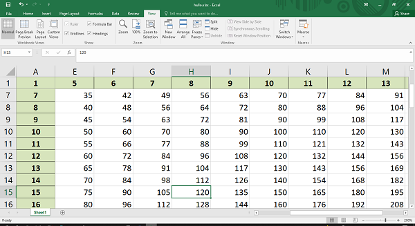
The split_panes() method
The split_panes() method also divides the worksheet into horizontal or vertical regions known as panes, but unlike freeze_panes() method, the splits between the panes will be visible to the user and each pane will have its own scroll bars.
The method has the parameters "y" and "x" that are used to specify the vertical and horizontal position of the split. These parameters are in terms of row height and column width used by Excel. The row heights and column widths have default values as 15 for a row and 8.43 for a column.
You can set one of the "y" and "x" parameters as zero if you do not want either a vertical or horizontal split.
To create a split at the 10th row and 7th column, the split_panes() method is used as follows −
worksheet.split_panes(15*10, 8.43*7)
You will find the splitters at 10th row and 7th column of the worksheet. You can scroll the panes to the left and right of vertical splitter and to the top and bottom of horizontal splitter. Note that the other panes will remain constant.
Example
Here's the complete code that creates the splitter, and below that the output is shown −
import xlsxwriter

wb = xlsxwriter.Workbook('hello.xlsx')
worksheet = wb.add_worksheet()
format1=wb.add_format({'bg_color':'#D9D9D9', 'bold':True})

for col in range(0, 15):
   worksheet.write(0, col, col+1, format1)

for row in range(1, 51):
   for col in range(0,15):
      if col==0:
         worksheet.write(row,col,(col+1)*(row + 1), format1)
      else:
         worksheet.write(row,col,(col+1)*(row + 1))
worksheet.split_panes(15*10, 8.43*7)

wb.close()
Output
Run the code and open hello.xlsx using Excel. As we can see, the worksheet is split into different panes at 10th row and 7th column.
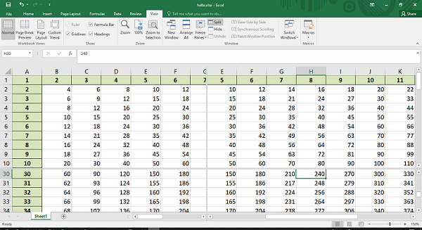
Python XlsxWriter - Hide/Protect Worksheet
The worksheet object's hide() method makes the worksheet disappear till it is unhidden through Excel menu.
In the following worksheet, there are three sheets, of which sheet2 is hidden.
sheet1 = workbook.add_worksheet()
sheet2 = workbook.add_worksheet()
sheet3 = workbook.add_worksheet()

# Hide Sheet2. It won't be visible until it is unhidden in Excel.
worksheet2.hide()
It will create the following worksheet −
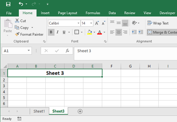
You can't hide the "active" worksheet, which generally is the first worksheet, since this would cause an Excel error. So, in order to hide the first sheet, you will need to activate another worksheet.
sheet2.activate()
sheet1.hide()
Hide Specific Rows or Columns
To hide specific rows or columns in a worksheet, set hidden parameter to 1 in set_row() or set_column() method. The following statement hides the columns C, D and E in the active worksheet.
worksheet.set_column('C:E', None, None, {'hidden': 1})
Example
Consider the following program −
import xlsxwriter

wb = xlsxwriter.Workbook('hello.xlsx')
worksheet = wb.add_worksheet()
format1=wb.add_format({'bg_color':'#D9D9D9', 'bold':True})

for col in range(0, 15):
   worksheet.write(0, col, col+1, format1)

for row in range(1, 51):
   for col in range(0,15):
      if col==0:
         worksheet.write(row,col,(col+1)*(row + 1), format1)
      else:
         worksheet.write(row,col,(col+1)*(row + 1))
worksheet.set_column('C:E', None, None, {'hidden': 1})

wb.close()
Output
As a result of executing the above code, the columns C, D and E are not visible in the worksheet below −
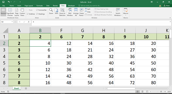
Similarly, we can hide rows with set_row() method with the help of hidden parameter.
for row in range(5, 7):
   worksheet.set_row(row, None, None, {'hidden':1})
Here is the result −
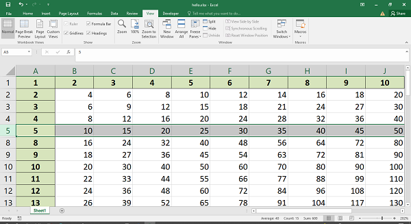
Python XlsxWriter - Textbox
In Excel, a text box is a graphic object that can be placed anywhere on the worksheet, and can be moved around if needed. Desired formatting features such as font (color, size, name etc.), alignment, fill effects, orientation etc. can be applied on the text contained in the text box.
Working with XlsxWriter Textbox
In XlsxWriter, there is insert_textbox() method to place text box on the worksheet. The cell location of the text box and the text to be written in it must be given. Additionally, different formatting options are given in the form of a dictionary object.
Example
The following code displays a text box at cell C5, the given string is displayed with font and alignment properties as shown below −
import xlsxwriter

wb = xlsxwriter.Workbook('hello.xlsx')
worksheet = wb.add_worksheet()
text = 'Welcome to TutorialsPoint'

options = {'font': {'color': 'red','size': 14},
   'align': {'vertical': 'middle','horizontal': 'center'}}
worksheet.insert_textbox('C5', text, options)

wb.close()
Output
Open the worksheet 'hello.xlsx' with Excel app. The text box appears as below −
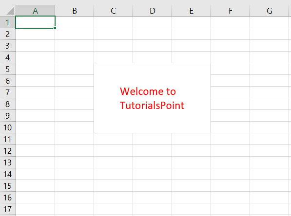
Textbox Options fill
The text box is by default 192X120 pixels in size (corresponds to 3 columns and 6 rows). This size can be changed with width and height parameters, both given in pixels. One of the parameters acceptable to inset_textbox() method is the fill parameter. It takes a predefined color name or color representation in hexadecimal as value.
Example
The following code displays a multi-line string in the custom sized text box having background filled with red color.
import xlsxwriter
wb = xlsxwriter.Workbook('hello.xlsx')
worksheet = wb.add_worksheet()
text = 'TutorialsPoint - Simple Easy Learning\nThe best resource for Online Education'

options = {
   'width': 384,
   'height':80,
   'font': {'color': 'blue', 'bold':True, 'size': 14},
   'align': {'vertical': 'middle', 'horizontal': 'center'},
   'fill':{'color':'red'},
}
worksheet.insert_textbox('C5', text, options)
wb.close()
As we can see in the figure below, a text box with multiple lines is rendered at cell C5.
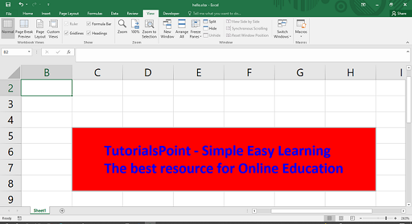
Textbox Options text_rotation
Another important property is the text_rotation. By default, the text appears horizontally. If required, you may change its orientation by giving an angle as its value. Look as the following options.
import xlsxwriter
wb = xlsxwriter.Workbook('hello.xlsx')
worksheet = wb.add_worksheet()
text = 'TutorialsPoint - Simple Easy Learning\nThe best resource for Online Education'

options = {
   'width': 128,
   'height':200,
   'font': {'bold':True, 'name':'Arial', 'size': 14},
   'text_rotation':90,
}
worksheet.insert_textbox('C5', text, options)
wb.close()
The text now appears in the text box with its vertical orientation.
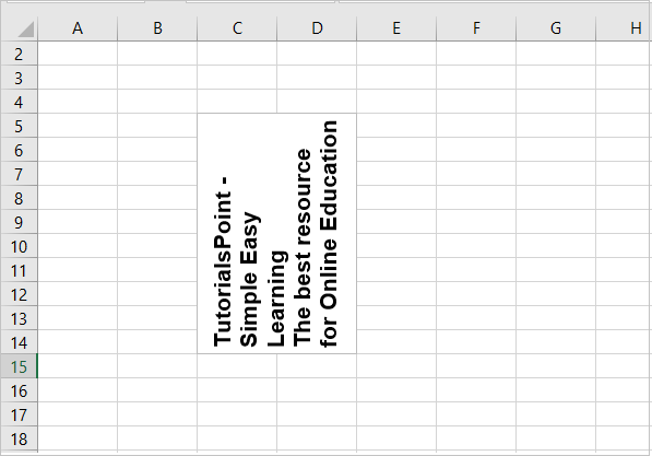
The object_position parameter controls the behaviour of the text box. It can have the following possible values and their effect −
"1" − Move and size with cells (the default).
"2" − Move but don't size with cells.
"3" − Don't move or size with cells.
Python XlsxWriter - Insert Image
It is possible to insert an image object at a certain cell location of the worksheet, with the help of insert_image() method. Basically, you have to specify the location of cell using any type of notation and the image to be inserted.
worksheet.insert_image('C5', 'logo.png')
The insert_image() method takes following optional parameters in a dictionary.
| Parameter | Default |
|---|---|
| 'x_offset' | 0, |
| 'y_offset' | 0, |
| 'x_scale' | 1, |
| 'y_scale' | 1, |
| 'object_position' | 2, |
| 'image_data' | None |
| 'url' | None |
| 'description' | None |
| 'decorative' | False |
The offset values are in pixels. The x_scale and y_scale parameters are used to scale the image horizontally and vertically.
The image_data parameter is used to add an in-memory byte stream in io.BytesIO format.
Example
The following program extracts the image data from a file in the current folder and uses is as value for image_data parameter.
from io import BytesIO
import xlsxwriter
workbook = xlsxwriter.Workbook('hello.xlsx')
worksheet = workbook.add_worksheet()

filename = 'logo.png'

file = open(filename, 'rb')
data = BytesIO(file.read())
file.close()

worksheet.insert_image('C5', filename, {'image_data': data})

workbook.close()
Output
Here is the view of the resultant worksheet −
Python XlsxWriter - Page Setup
The worksheet page setup methods are related to appearance of the worksheet when it is printed. These worksheet methods control the orientation, paper size, margins, etc.
set_landscape()
This method is used to set the orientation of a worksheet's printed page to landscape.
set_portrait()
This method is used to set the orientation of a worksheet's printed page to portrait. This is the default orientation.
set_page_view()
This method is used to display the worksheet in "Page View/Layout" mode.
set_paper()
This method is used to set the paper format for the printed output of a worksheet. It takes index as an integer argument. It is the Excel paper format index.
Following are some of the paper styles and index values −
| Index | Paper format | Paper size |
|---|---|---|
| 0 | Printer default | Printer default |
| 1 | Letter | 8 1/2 x 11 in |
| 2 | Letter Small | 8 1/2 x 11 in |
| 3 | Tabloid | 11 x 17 in |
| 4 | Ledger | 17 x 11 in |
| 5 | Legal | 8 1/2 x 14 in |
| 6 | Statement | 5 1/2 x 8 1/2 in |
| 7 | Executive | 7 1/4 x 10 1/2 in |
| 8 | A3 | 297 x 420 mm |
| 9 | A4 | 210 x 297 mm |
set_margin()
This method is used to set the margins of the worksheet when it is printed. It accepts left, right, top and bottom parameters whose values are in inches. All parameters are optional The left and right parameters are 0.7 by default, and top and bottom are 0.75 by default.
Python XlsxWriter - Header & Footer
When the worksheet is printed using the above methods, the header and footer are generated on the paper. The print preview also displays the header and footer. Both are configured with set_header() and set_footer() methods. Header and footer string is configured by following control characters −
| Control | Category | Description |
|---|---|---|
| &L | Justification | Left |
| &C | Center | |
| &R | Right | |
| &P | Information | Page number |
| &N | Total number of pages | |
| &D | Date | |
| &T | Time | |
| &F | File name | |
| &A | Worksheet name | |
| &Z | Workbook path | |
| &fontsize | Font | Font size |
| &"font,style" | Font name and style | |
| &U | Single underline | |
| &E | Double underline | |
| &S | Strikethrough | |
| &X | Superscript | |
| &Y | Subscript | |
| &[Picture] | Images | Image placeholder |
| &G | Same as &[Picture] | |
| && | Misc. | Literal ampersand "&" |
Example
The following code uses set_header() and set_footer() methods −
import xlsxwriter

wb = xlsxwriter.Workbook('hello.xlsx')
ws = wb.add_worksheet()

data = [
   ['Anil', 45, 55, 50], ['Ravi', 60, 70, 80],
   ['Kiran', 65, 75, 85],['Karishma', 55, 65, 45]
]

for row in range(len(data)):
   ws.write_row(row,0, data[row])

header1 = '&CTutorialspoint'
footer1 = '&LSimply Easy Learning'

ws.set_landscape()
ws.set_paper(9) #A4 paper
ws.set_header(header1)
ws.set_footer(footer1)

ws.set_column('A:A', 50)

wb.close()
Output
Run the above Python code and open the worksheet. From File menu, choose Print option. On the right pane, the preview is shown. You should be able to see the header and footer.
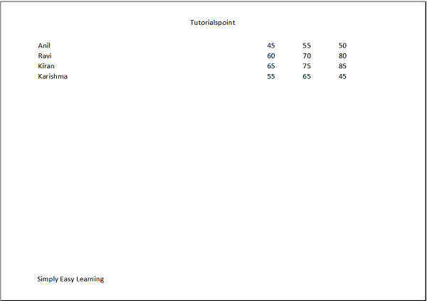
Python XlsxWriter - Cell Comments
In an Excel worksheet, comments can be inserted for various reasons. One of the uses is to explain a formula in a cell. Also, Excel comments also serve as reminders or notes for other users. They are useful for cross-referencing with other Excel workbooks.
From Excel's menu system, comment feature is available on Review menu in the ribbon.
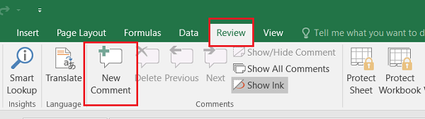
To add and format comments, XlsxWriter has add_comment() method. Two mandatory parameters for this method are cell location (either in A1 type or row and column number), and the comment text.
Example
Here is a simple example −
import xlsxwriter

wb = xlsxwriter.Workbook('hello.xlsx')
ws = wb.add_worksheet()

data='XlsxWriter Library'

ws.set_column('C:C', 25)
ws.set_row(2, 50)
ws.write('C3', data)

text = 'Developed by John McNamara'
ws.write_comment('C3', text)

wb.close()
Output
When we open the workbook, a comment will be seen with a marker on top right corner of C3 cell when the cursor is placed in it.
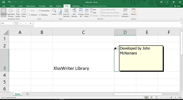
By default, the comments are not visible until the cursor hovers on the cell in which the comment is written. You can either show all the comments in a worksheet by invoking show_comment() method of worksheet object, or setting visible property of individual comment to True.
ws.write_comment('C3', text, {'visible': True})
Example
In the following code, there are three comments placed. However, the one in cell C3 is has been configured with visible property set to False. Hence, it cannot be seen until the cursor is placed in the cell.
import xlsxwriter

wb = xlsxwriter.Workbook('hello.xlsx')
ws = wb.add_worksheet()

ws.show_comments()

data='Python'
ws.set_column('C:C', 25)
ws.set_row(0, 50)
ws.write('C1', data)
text = 'Programming language developed by Guido Van Rossum'
ws.write_comment('C1', text)
data= 'XlsxWriter'
ws.set_row(2, 50)
ws.write('C3', data)
text = 'Developed by John McNamara'
ws.write_comment('C3', text, {'visible':False})
data= 'OpenPyXl'
ws.set_row(4, 50)
ws.write('C5', data)
text = 'Developed by Eric Gazoni and Charlie Clark'
ws.write_comment('C5', text, {'visible':True})

wb.close()
Output
It will produce the following output −
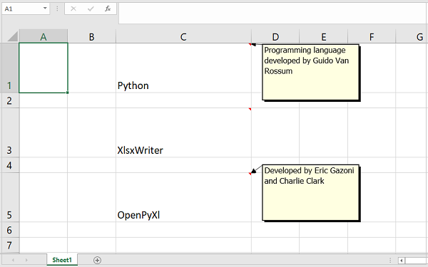
You can set author option to indicate who is the author of the cell comment. The author of the comment is also displayed in the status bar at the bottom of the worksheet.
worksheet.write_comment('C3', 'Atonement', {'author': 'Tutorialspoint'})
The default author for all cell comments can be set using the set_comments_author() method −
worksheet.set_comments_author('Tutorialspoint')
It will produce the following output −
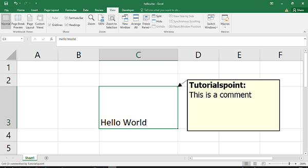
Python XlsxWriter - Working with Pandas
Pandas is a popular Python library for data manipulation and analysis. We can use XlsWriter for writing Pandas dataframes into an Excel worksheet.
To learn the features described in this section, we need to install Pandas library in the same environment in which XlsxWriter has been installed.
pip3 install pandas
Using XlsxWriter with Pandas
Let us start with a simple example. First, create a Pandas dataframe from the data from a list of integers. Then use XlsxWriter as the engine to create a Pandas Excel writer. With the help of this engine object, we can write the dataframe object to Excel worksheet.
Example
import pandas as pd

df = pd.DataFrame({'Data': [10, 20, 30, 20, 15, 30, 45]})
writer = pd.ExcelWriter('hello.xlsx', engine='xlsxwriter')
df.to_excel(writer, sheet_name='Sheet1')

writer.save()
Output
The worksheet so created shows up as follows −
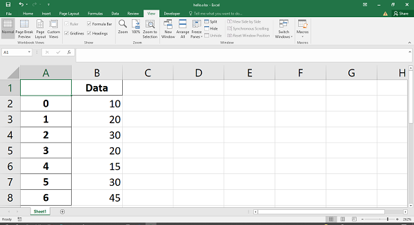
Adding Charts to Pandas Dataframe
Just as we obtain an object of Workbook class, and then a Worksheet object by calling its add_worksheet() method, the writer object can also be used to fetch these objects. Once we get them, the XlsxWriter methods to add chart, data table etc. can be employed.
In this example, we set up a Pandas dataframe and obtain its dimension (or shape).
import pandas as pd
df = pd.DataFrame({'Data': [105, 60, 35, 90, 15, 30, 75]})
writer = pd.ExcelWriter('hello.xlsx', engine='xlsxwriter')
df.to_excel(writer, sheet_name='Sheet1')
(max_row, max_col) = df.shape
The workbook and worksheet objects are created from the writer.
workbook = writer.book
worksheet = writer.sheets['Sheet1']
Rest of things are easy. The chart object is added as we have done earlier.
chart = workbook.add_chart({'type': 'column'})
chart.add_series({'values': ['Sheet1', 1, 1, max_row, 1]})
worksheet.insert_chart(1, 3, chart)
writer.save()
Example
The following code uses Pandas dataframe to write an Excel workbook and a column chart is prepared by XlsxWriter.
import pandas as pd

df = pd.DataFrame({'Data': [105, 60, 35, 90, 15, 30, 75]})
writer = pd.ExcelWriter('hello.xlsx', engine='xlsxwriter')
df.to_excel(writer, sheet_name='Sheet1')
(max_row, max_col) = df.shape

workbook = writer.book
worksheet = writer.sheets['Sheet1']
chart = workbook.add_chart({'type': 'column'})
chart.add_series({'values': ['Sheet1', 1, 1, max_row, 1]})
worksheet.insert_chart(1, 3, chart)

writer.save()
Output
The column chart along with the data is shown below −
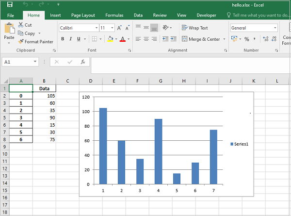
Writing Dataframe to Excel Table
Similarly, the dataframe can be written to Excel table object. The dataframe here is derived from a Python dictionary, where the keys are dataframe column headers. Each key has list as a value which in turn becomes values of each column.
import pandas as pd

df = pd.DataFrame({
   'Name': ['Namrata','Ravi','Kiran','Karishma'],
   'Percent': [73.33, 70, 75, 65.5],
   'RollNo': [1, 2,3,4]})

df = df[['RollNo', 'Name', 'Percent']]
(max_row, max_col) = df.shape
Use xlsxwriter engine to write the dataframe to a worksheet (sheet1)
writer = pd.ExcelWriter('hello.xlsx', engine='xlsxwriter')
df.to_excel(writer, sheet_name='Sheet1', startrow=1, header=False, index=False)
Following lines give Workbook and Worksheet objects.
workbook = writer.book
worksheet = writer.sheets['Sheet1']
Data in the worksheet is converted to Table with the help of add_table() method.
column_settings = [{'header': column} for column in df.columns]

worksheet.add_table(0, 0, max_row, max_col - 1, {'columns': column_settings})

writer.save()
Example
Below is the complete code to write pandas dataframe to Excel table.
import pandas as pd
df = pd.DataFrame({
   'Name': ['Namrata','Ravi','Kiran','Karishma'],
   'Percent': [73.33, 70, 75, 65.5],
   'RollNo': [1, 2,3,4]
})

df = df[['RollNo', 'Name', 'Percent']]
(max_row, max_col) = df.shape

writer = pd.ExcelWriter('hello.xlsx', engine='xlsxwriter')
df.to_excel(writer, sheet_name='Sheet1', startrow=1, header=False, index=False)

workbook = writer.book
worksheet = writer.sheets['Sheet1']

column_settings = [{'header': column} for column in df.columns]

worksheet.add_table(0, 0, max_row, max_col - 1, {'columns': column_settings})

writer.save()
Output
The Table using default autofilter settings appears at A1 cell onwards.
Python XlsxWriter - VBA Macro
In Excel, a macro is a recorded series of steps that can be repeated any number of times with a shortcut key. The steps performed while recording the macro are translated into programming instructions VBA which stands for Visual Basic for Applications. VBA is a subset of Visual basic language, especially written to automate the tasks in MS Office apps such as Word, Excel, PowerPoint etc.
The option to record a macro is available in the Developer menu of MS Excel. If this menu is not seen, it has to be activated by going to the "File→Options→Customize" ribbon screen.
As shown in the following figure, click the Record Macro button by going to "View→Macros→Record Macro", and give a suitable name to the macro and perform desired actions to be recorded. After the steps are over stop the recording. Assign a desired shortcut so that the recorded action can be repeated as and it is pressed.
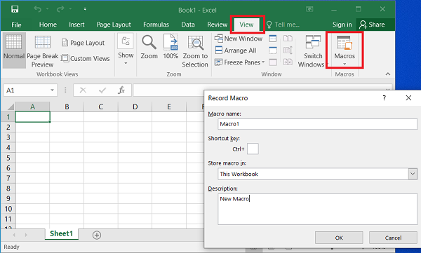
To view the VBA code, edit the macro by going View→ZMacros→View Macros. Select the Macro from Macro name and click on Edit.
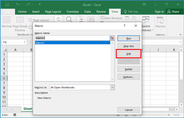
The VBA editor will be shown. Delete all the steps generated by Excel and add the statement to pop-up a message box.
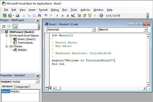
Confirm that the macro works perfectly. Press CTL+Shift+M and the message box pops up. Save this file with the .xlsm extension. It internally contains vbaproject.bin, a binary OLE COM container. To extract it from the Excel macro file, use the vba_extract.py utility.
(xlsxenv) E:\xlsxenv>vba_extract.py test.xlsm
Extracted: vbaProject.bin
Example
This vbaProject.bin file can now be added to the XlsxWriter workbook using the add_vba_project() method. On this worksheet, place a button object at B3 cell, and link it to the macro that we had already created (i.e., macro1)
import xlsxwriter

workbook = xlsxwriter.Workbook('testvba.xlsm')
worksheet = workbook.add_worksheet()

worksheet.set_column('A:A', 30)
workbook.add_vba_project('./vbaProject.bin')
worksheet.write('A3', 'Press the button to say Welcome.')
worksheet.insert_button(
   'B3',
   {
      'macro': 'macro1',
      'caption': 'Press Me',
      'width': 80, 'height': 30
   }
)
workbook.close()
Output
When the above code is executed, the macro enabled workbook named testvba.xlsm will be created. Open it and click on the button. It will cause the message box to pop up as shown.