MATLAB - Polynomial Addition

In mathematics, a polynomial is an expression consisting of variables (also called indeterminates) and coefficients, that involves only the operations of addition, subtraction, multiplication, and non-negative integer exponents of variables. For example, 3x2 - 2x + 1 is a polynomial in the variable x.

Polynomials can be represented in MATLAB using arrays, where the elements of the array correspond to the coefficients of the polynomial terms. For example, the polynomial 3x2 - 2x + 1 can be represented as p = [3, -2, 1] in MATLAB.

To add two polynomials in MATLAB, you can simply add the corresponding coefficients of the polynomials. For example, to add the polynomials 3x2 - 2x + 1 and 2x2 + 4x - 3, you would add the coefficients to get the result polynomial.

Polynomial representation in Matlab

In MATLAB, polynomials are represented using row vectors where the elements correspond to the coefficients of the polynomial terms. These coefficients, denoted as a1,a2,a3.aN , represent the coefficients of x raised to successive powers.

The first element in the vector represents the coefficient of x with the highest power, and subsequent elements correspond to lower powers of x. It's important to include all coefficients in the vector, even those that are equal to zero.

For example the polynomial : −

p(x) = 4x5 + 5x2 - 2x + 7

Can be represented in Matlab as : −

p = [4  0  0  5  -2  7]

To understand it further , In MATLAB, the elements of the row vector p represent the coefficients of the polynomial terms in descending order of their powers of x.Here's how each coefficient corresponds to the power of x in the polynomial.

• The coefficient 4 corresponds to the term 4x5, indicating that the coefficient of x5 is 4.
• The coefficients 0, 0 represent the terms 0x4 and 0x3.Even though these terms are absent in the given polynomial, they are included with zero coefficients to maintain the order of powers.
• The coefficients 0, 0 represent the terms 0x4 and 0x3.Even though these terms are absent in the given polynomial, they are included with zero coefficients to maintain the order of powers.
• The coefficient 5 corresponds to the term 5x2, indicating that the coefficient of x2 is 5.
• The coefficient -2 corresponds to the term -2x, indicating that the coefficient of x1 (which is just x) is -2.
• The coefficient 7 corresponds to the constant term, indicating that the coefficient of x0, (which is just the constant) is 7.

So, the row vector p [4 0 0 5 -2 7] represents the polynomial

p(x) = 4x5 + 5x2 - 2x + 7

in Matlab. Each element of the vector corresponds to a coefficient of a specific power of x, and zero coefficients are included for any missing terms to maintain the correct order.

Adding Polynomials in Matlab

To add two polynomials in MATLAB, you can use the arithmetic operator plus '+'. For instance, if you have two polynomials x and y, you can add them using the command.

z = x + y;

In this operation, MATLAB adds the corresponding elements of the row vectors x and y to produce the result in the vector z. Each element of z will be the sum of the coefficients of the corresponding terms in x and y.

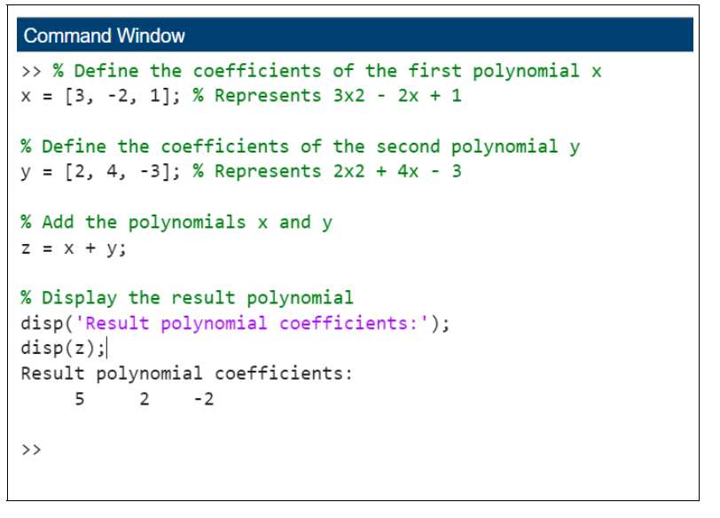
Here is a more detailed explanation with an example −

% Define the coefficients of the first polynomial x
x = [3, -2, 1]; % Represents 3x2 - 2x + 1

% Define the coefficients of the second polynomial y
y = [2, 4, -3]; % Represents 2x2 + 4x - 3

% Add the polynomials x and y
z = x + y;

% Display the result polynomial
disp('Result polynomial coefficients:');
disp(z);

In this example, the polynomials x and y are added to get the result polynomial z. The result z will be [5, 2, -2], which corresponds to the polynomial 5x2 + 2x - 2, the sum of the two input polynomials.

Following is the output of the above code −

Let us try few more similar examples as shown below.

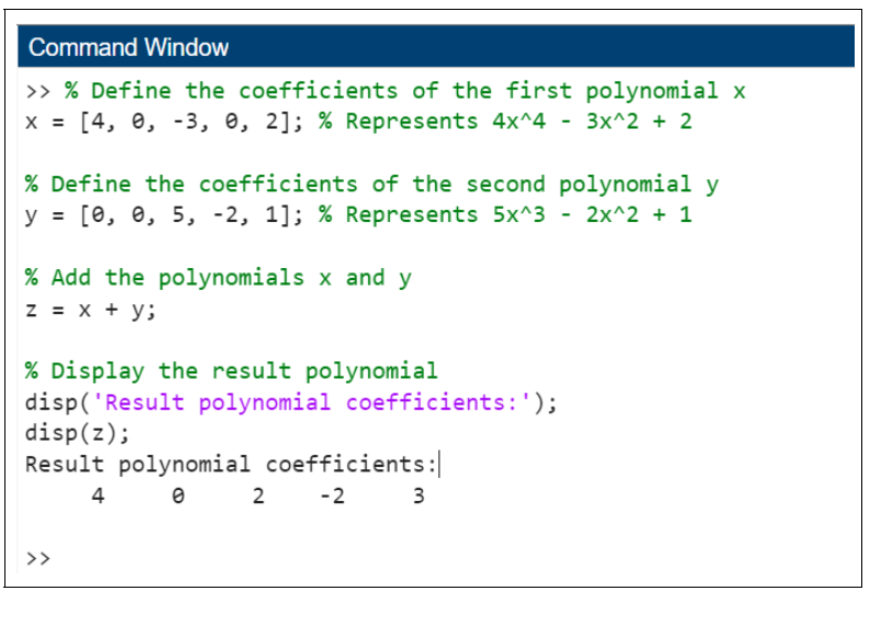
Example: Adding polynomial 4x4 - 3x2 + 2 and 5x3 - 2x2 + 1

The code we have is

% Define the coefficients of the first polynomial x
x = [4, 0, -3, 0, 2]; % Represents 4x4 - 3x2 + 2

% Define the coefficients of the second polynomial y
y = [0, 0, 5, -2, 1]; % Represents 5x3 - 2x2 + 1

% Add the polynomials x and y
z = x + y;

% Display the result polynomial
disp('Result polynomial coefficients:');
disp(z);

When the code is executed the output we get is −

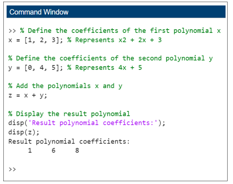
Example: Adding polynomial x2 + 2x + 3 and 4x + 5

The code we have is −

% Define the coefficients of the first polynomial x
x = [1, 2, 3]; % Represents x2 + 2x + 3

% Define the coefficients of the second polynomial y
y = [0, 4, 5]; % Represents 4x + 5

% Add the polynomials x and y
z = x + y;

% Display the result polynomial
disp('Result polynomial coefficients:');
disp(z);

When the code is executed the output we get is as follows −