Seaborn.scatterplot() method

The Seaborn.scatterplot() method helps to draw a scatter plot with the possibility of several semantic groupings. That is variables can be grouped and a graphical representation of these variables can be drawn.

Scatter plot is an example of a graph, which is a data visualization tool, that is used to represent the relationship between any two points in a set of datapoints. They are used to plot two-dimensional graphics that can be enhanced with the help of hue, size and style parameters. This plot can be mapped upto three variables independently but this plot is hard to interpret and often ineffective. We can use redundant semantics in this case to make graphics more accessible.

Syntax

The syntax of the seaborn.scatterplot() function is as follows.

seaborn.scatterplot(*, x=None, y=None, hue=None, style=None, size=None, data=None, palette=None, hue_order=None, hue_norm=None, sizes=None, size_order=None, size_norm=None, markers=True, style_order=None, x_bins=None, y_bins=None, units=None, estimator=None, ci=95, n_boot=1000, alpha=None, x_jitter=None, y_jitter=None, legend='auto', ax=None, **kwargs)

Parameters

Some of the parameters of the scatterplot() method are discussed below.

S.No	Parameter and Description
1	x,y Variables that are represented on the x,y axis.
2	Hue This will produce elements with different colors. It is a grouping variable.
3	Size This will produce elements with different sizes. It is also a grouping variable.
4	Style This will produce elements with different styles.
5	Data This parameter takes the input data structure. That is either a mapping or a sequence.
7	Hue_order Order of plotting categorical variables in hue semantic.
8	Kind Corresponds to the kind of plot to be drawn. Can be line or scatter. Scatter plot is the default setting.
9	Palette This parameter is used to set the color tone of the mapping. It can be bright, pastel, dark etc.
10	Height, width These are scalar quantities that determine the height and width of the plot.
11	Legend() Can be “auto”,”brief”,”full” or “false”. Depending on the value given, the groups will be placed in the legend.
12	Ci() Size of the confidence interval when aggregating the estimator.

Return Value

The scatterplot() method returns the matplotlib axes containing the plotted points.

Loading the Seaborn library

Let us load the Seaborn library and the dataset before moving on to developing the plots. To load or import the Seaborn library the following line of code can be used.

Import seaborn as sns

Loading the dataset

in this article, we will make use of the Titanic dataset inbuilt into the Seaborn library. the following command is used to load the dataset.

dts=sns.load_dataset("titanic")

The below-mentioned command is used to view the first 5 rows in the dataset. This enables us to understand what variables can be used to plot a graph.

dts.head()

Following is the output for the above piece of code.

index,survived,pclass,sex,age,sibsp,parch,fare,embarked,class,who,adult_male,deck,embark_town,alive,alone
0,0,3,male,22.0,1,0,7.25,S,Third,man,true,NaN,Southampton,no,false
1,1,1,female,38.0,1,0,71.2833,C,First,woman,false,C,Cherbourg,yes,false
2,1,3,female,26.0,0,0,7.925,S,Third,woman,false,NaN,Southampton,yes,true

Example 1

This first example will show how to draw a basic scatterplot using three parameters in the function.

import seaborn as sns
import matplotlib.pyplot as plt
dts=sns.load_dataset("titanic")
dts.head()
sns.scatterplot(data=dts,x="age",y="fare",hue="sex")
plt.show()

Output

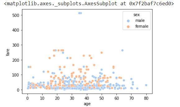
Here, the graph is plotted as a relation between the age and fare for the genders male and female.

Changing the palette color

To change the palette color for your plots, the following line of code can be used.

sns.set_palette("muted")

Example 2

This example will show the usage of 4 parameters in the scatterplot() method.

For this dataset, this plot helps to view the variation between the age and fare of different genders for different classes of people.

import seaborn as sns
import matplotlib.pyplot as plt
dts=sns.load_dataset("titanic")
dts.head()
sns.scatterplot(data=dts,x="age",y="fare",hue="class",style="sex")
plt.show()

Output

Example 3

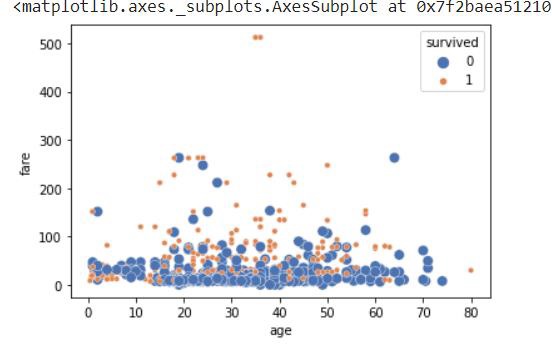
In this example, we will understand how to use parameters legend and sizes. Legend is the parameter that determines what data should be placed in the legend. If it is full, all the groups will get placed in the legend else, only some will get placed. So in this example, all the groups in the dataset will get placed in the legend.

Sizes determine how the sizes are chosen for the “size” parameter. So in this example, sizes are minimum 20 and maximum 70. Which means for the size parameter, the data points displayed will vary in this size range.

import seaborn as sns
import matplotlib.pyplot as plt
dts=sns.load_dataset("titanic")
dts.head()
sns.scatterplot( data=dts, x="age", y="fare", hue="survived",size="survived", sizes=(20, 70), legend="full" )
plt.show()

Output

Example 4

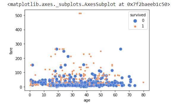
In this example, we will pass a new parameter hue_norm which will take either numerical or string values. It basically is used to specify the order of processing and plotting of the categorical variable given in the “hue” parameter.

The hue_norm value we use is (0,3). This means that for survived variable, the values are given from 0 to 3 depending on the values of the survived column in the dataset.

import seaborn as sns
import matplotlib.pyplot as plt
dts=sns.load_dataset("titanic")
dts.head()
sns.scatterplot(
data=dts, x="age", y="fare", hue="survived", size="survived",
sizes=(20, 70),hue_norm=(0, 3), legend="full",palette="deep"
)
plt.show()

Output

seaborn_relational_plots_introduction.htm