- Seaborn - Home
- Seaborn - Introduction
- Seaborn - Environment Setup
- Importing Datasets and Libraries
- Seaborn - Figure Aesthetic
- Seaborn- Color Palette
- Seaborn - Histogram
- Seaborn - Kernel Density Estimates
- Visualizing Pairwise Relationship
- Seaborn - Plotting Categorical Data
- Distribution of Observations
- Seaborn - Statistical Estimation
- Seaborn - Plotting Wide Form Data
- Multi Panel Categorical Plots
- Seaborn - Linear Relationships
- Seaborn - Facet Grid
- Seaborn - Pair Grid
- Seaborn Useful Resources
- Seaborn - Quick Guide
- Seaborn - cheatsheet
- Seaborn - Useful Resources
- Seaborn - Discussion
Seaborn.residplot() method
The Seaborn.residplot() method is used to plot residual data of a linear regression. This function will do a robust or polynomial regression on the variables y and x and then plot the residuals as a scatterplot. If you want to see if the residuals have any structure, you can choose to fit a lowess smoother to the residual plot.
A residual plot is a graph data visualization tool that plots the residual points on the y-axis and the independent factors on the x-axis. This tool determines whether the regression model applied on the points has to be linear or non-linear.
Syntax
Following is the syntax of the seaborn.residplot() method −
seaborn.residplot(*, x=None, y=None, data=None, lowess=False, x_partial=None, y_partial=None, order=1, robust=False, dropna=True, label=None, color=None, scatter_kws=None, line_kws=None, ax=None
Parameters
Some of the parameters of the residplot() method are discussed below.
| S.No | Parameter and Description |
|---|---|
| 1 | x,y These parameters take names of variables as input that plot the long form data. Input can be either a vector or a string. |
| 2 | data This is the dataframe that is used to plot graphs. |
| 3 | Lowess This parameter takes Boolean values and fits a lowess smoother to the residual scatterplot. |
| 4 | {x,y}_partial This optional parameter accepts texts or matrices as input. The input is either the column name in the data, or a matrix with the same first dimension as x. Before plotting, these variables are considered as confounding and subtracted from the x or y variables. |
| 5 | Order This optional parameter accepts integer values and determines the order of the polynomial to fit when calculating the residuals. |
| 6 | Color Used to specify a single color, and this color is applied to all plot elements. |
| 7 | robust This optional parameter takes Boolean values and fits a robust linear regression when calculating the residuals. |
| 8 | dropna It takes Boolean values and if True, ignore observations with missing data. |
Return value
The residplot() method returns the matplotlib axes with plotted points.
Loading the seaborn library
Let us load the seaborn library and the dataset before moving on to developing the plots. To load or import the seaborn library the following line of code can be used.
Import seaborn as sns
Loading the dataset
In this article, we will make use of the Titanic dataset inbuilt in the seaborn library. the following command is used to load the dataset.
titanic=sns.load_dataset("titanic")
The below mentioned command is used to view the first 5 rows in the dataset. This enables us to understand what variables can be used to plot a graph.
titanic.head()
The below is the output for the above piece of code.
index,survived,pclass,sex,age,sibsp,parch,fare,embarked,class,who,adult_male,deck,embark_town,alive,alone
0,0,3,male,22.0,1,0,7.25,S,Third,man,true,NaN,Southampton,no,false
1,1,1,female,38.0,1,0,71.2833,C,First,woman,false,C,Cherbourg,yes,false
2,1,3,female,26.0,0,0,7.925,S,Third,woman,false,NaN,Southampton,yes,true
Now that we have loaded the dataset, we will explore as few examples.
Example 1
We will use the titanic dataset in this article and to plot a residplot() we will pass the age and survived columns of the dataset to the x,y parameters and change the color of the plot by passing the color parameter to the seaborn.residplot() method. In this case we are passing the string g to the color and this changes the plot to green color.
import seaborn as sns
import matplotlib.pyplot as plt
titanic=sns.load_dataset("titanic")
titanic.head()
sns.residplot(y="survived", x="age",color="g",data=titanic)
plt.show()
Output
The output obtained is as follows,

Example 2
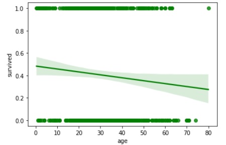
Now we will understand the usage of the robust parameter. This optional parameter takes Boolean values and fits a robust linear regression when calculating the residuals. The way that this parameter is used is depicted below. In the below example, robust is passed True.
import seaborn as sns
import matplotlib.pyplot as plt
titanic=sns.load_dataset("titanic")
titanic.head()
sns.regplot(y="survived", x="age",color="g", robust=True,data=titanic)
plt.show()
Output
the output of the plot is as follows,
Example 3
Lowess is another parameter in the seaborn.residplot() method which is used often. This parameter takes Boolean values and fits a lowess smoother to the residual scatterplot.
Since we are using the titanic dataset in this article and to plot a residplot() we will pass the age and survived columns of the dataset to the x,y parameters respectively. We are passing the Boolean value True to the lowess parameter and the color red, e+ie: the string r is being passed to the color attribute which changes the plot to a red color.
The plot can be observed below.
import seaborn as sns
import matplotlib.pyplot as plt
titanic=sns.load_dataset("titanic")
titanic.head()
sns.regplot(y="survived", x="age",color="r", lowess=True,data=titanic)
plt.show()
Output
the plot obtained is,
