- Seaborn - Home
- Seaborn - Introduction
- Seaborn - Environment Setup
- Importing Datasets and Libraries
- Seaborn - Figure Aesthetic
- Seaborn- Color Palette
- Seaborn - Histogram
- Seaborn - Kernel Density Estimates
- Visualizing Pairwise Relationship
- Seaborn - Plotting Categorical Data
- Distribution of Observations
- Seaborn - Statistical Estimation
- Seaborn - Plotting Wide Form Data
- Multi Panel Categorical Plots
- Seaborn - Linear Relationships
- Seaborn - Facet Grid
- Seaborn - Pair Grid
- Seaborn Useful Resources
- Seaborn - Quick Guide
- Seaborn - cheatsheet
- Seaborn - Useful Resources
- Seaborn - Discussion
Seaborn.kdeplot() method
The Seaborn.kdeplot() method helps to plot univariate or bivariate distributions using a kernel density estimation.
Similar to a histogram, a kernel density estimate plot is a technique for displaying the distribution of observations in a dataset. Kernel Density Estimate (KDE) uses a continuous probability density curve in one or more dimensions to describe the data.
Syntax
Following is the syntax of the Seaborn.kdeplot() method
Seaborn.kdeplot(x=None, *, y=None, shade=None, vertical=False, kernel=None, bw=None, gridsize=200, cut=3, clip=None, legend=True, cumulative=False, shade_lowest=None, cbar=False, cbar_ax=None, cbar_kws=None, ax=None, weights=None, hue=None, palette=None, hue_order=None, hue_norm=None, multiple='layer', common_norm=True, common_grid=False, levels=10, thresh=0.05, bw_method='scott', bw_adjust=1, log_scale=None, color=None, fill=None, data=None, data2=None, warn_singular=True, **kwargs)
Parameters
Some of the parameters of the seaborn.kdeplot() method are discussed below.
| S.No | Parameter and Description |
|---|---|
| 1 | x,y Variables that are represented on the x,y axis. |
| 2 | Hue This will produce elements with different colors. It is a grouping variable. |
| 3 | Levels This parameter is used to specify the number of levels to draw contours at in the graph. |
| 4 | Cmap Cmap or color map is used to specify the colors to be used in plotting the map. Takes different kinds of values such as blues, greens, PiYg etc. |
| 5 | Bw_adjust Takes numerical values and smoothens the curve plotted as the value passed increases. |
| 6 | Thresh Is used to specify the lowest level at which to draw a contour at. Takes values from 0 to 1. |
| 7 | Cumulative Plots the cumulative count as number of bins increase. |
| 8 | Multiple Related to univariate data and takes values: stacked, layer and fill. |
| 9 | Log_scale Sets axes scales to log and the values plotted are in log scale. |
| 10 | Legend Boolean value. If false, does not print out the legend of semantic variables. |
let us load the Seaborn library and the dataset before moving on to the developing the plots.
Loading the Seaborn library
To load or import the Seaborn library the following line of code can be used.
Import seaborn as sns
What kind of data is needed?
Bivariate data is needed to understand most of the parameters that are part of the kdeplot() method. Although, this method provides ways to plot kdeplot() for univariate data, it has more parameters to plot bivariate data and for this reason the flights dataset is considered since it contains bivariate data.
(Bivariate data means that the data is dependent on more than one variable and univariate data means that data is dependent only on one variable.)
Loading the dataset
in this article, we will make use of the flights dataset inbuilt in the seaborn library. the following command is used to load the dataset.
flights=sns.load_dataset("flights")
The below mentioned command is used to view the first 5 rows in the dataset. This enables us to understand what variables can be used to plot a graph.
flights.head()
the below is the output for the above piece of code.
index,year,month,passengers
0,1949,Jan,112
1,1949,Feb,118
2,1949,Mar,132
3,1949,Apr,129
4,1949,May,121
Now that we have loaded the data, we will move on to plotting the data.
Example 1
In this example, we will see how to plot a kernel density estimate for each column in a wide-form dataset using the seaborn.kdeplot() method. To do so, the following line of code can be used.
import seaborn as sns
import matplotlib.pyplot as plt
flights=sns.load_dataset("flights")
flights.head()
sns.kdeplot(data=flights)
plt.show()
Output
the output graph for the above code is given below.

Example 2
Now, we will see how to plot a basic kdeplot for the given dataset.
import seaborn as sns
import matplotlib.pyplot as plt
flights=sns.load_dataset("flights")
flights.head()
sns.kdeplot(data=flights, x="year", y="passengers")
plt.show()
Output
the output plot for the above code snippet can be seen below.

Example 3
In this example, we will see how the fill parameter can be used. So, this parameter is used to fill color in the contours of the graph defined. In the below code, x,y and hue parameters are considered and the graph thus obtained is filled with color since True is passed to the fil parameter.
import seaborn as sns
import matplotlib.pyplot as plt
flights=sns.load_dataset("flights")
flights.head()
sns.kdeplot(data=flights, x="year", y="passengers",fill=True,hue="month")
plt.show()
Output
the output of the above code snippet is as follows,
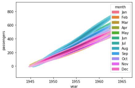
Here, as stated above, the contours of the graph are filled.
Example 4
We will understand the levels parameter in this example. Levels parameter takes the number of contour levels to be drawn in the graph and it can be either an integer or a vector value. This parameter is relevant only in the case of bivariate data. Here, cmap parameter is used to change the color of the plot. The cmap parameter can take different values and in this example, PiYG is passed to it and the colors produced range from pink to green. Some other values that the cmap can take include, blues, greens etc.
import seaborn as sns
import matplotlib.pyplot as plt
flights=sns.load_dataset("flights")
flights.head()
sns.kdeplot(data=flights, x="year", y="passengers",levels=10, cmap="PiYG")
plt.show()
Output
the plot obtained by using the above parameter can be seen below.

This is how the kdeplot() method can be used along with the usage of its parameters.