- Julia - Home
- Julia - Overview
- Julia - Environment Setup
- Julia - Basic Syntax
- Julia - Arrays
- Julia - Tuples
- Integers & Floating-Point Numbers
- Julia - Rational & Complex Numbers
- Julia - Basic Operators
- Basic Mathematical Functions
- Julia - Strings
- Julia - Functions
- Julia - Flow Control
- Julia - Dictionaries & Sets
- Julia - Date & Time
- Julia - Files I/O
- Julia - Metaprogramming
- Julia - Plotting
- Julia - Data Frames
- Working with Datasets
- Julia - Modules and Packages
- Working with Graphics
- Julia - Networking
- Julia - Databases
- Julia Useful Resources
- Julia - Quick Guide
- Julia - Useful Resources
- Julia - Cheatsheet
- Julia - Discussion
Julia - Quick Guide
Julia - Overview
What is Julia Programming Language?
One of the facts about scientific programming is that it requires high performance flexible dynamic programming language. Unfortunately, to a great extent, the domain experts have moved to slower dynamic programming languages. There can be many good reasons for using such dynamic programming languages and, in fact, their use cannot be diminished as well. On the flip side, what can we expect from modern language design and compiler techniques? Some of the expectations are as follows −
It should eradicate the performance trade-off.
It should provide the domain experts a single environment that is productive enough for prototyping.
It should provide the domain experts a single environment that is efficient enough for deploying performance-intensive applications.
The Julia programming language fulfills these expectations. It is a general purpose high-performance flexible programming language which can be used to write any application. It is well-suited for scientific and numerical computing.
History of Julia
Let us see the history of Julia programming language in the following points −
Jeff Bezanson, Stefan Karpinski, Viral B. Shah, and Alan Edelman has started to work on Julia in 2009.
The developers team of above four has launched a website on 14th February 2012. This website had a blog post primarily explaining the mission of Julia programming language.
Later in April 2012, Stefan Karpinski, in an interview with a magazine named InfoWorld, gave the name Julia for their programming language.
In 2014, the annual academic conference named The JuliaCon for Julia; users and developers has been started and since then it was regularly held every year.
In August 2014, Julia Version 0.3 was released for use.
In October 2015, Julia Version 0.4 was released for use.
In October 2016, Julia Version 0.5 was released for use.
In June 2017 Julia Version 0.6 was released for use.
Julia Version 0.7 and Version 1.0 were both released on the same date 8th August 2018. Among them Julia version 0.7 was particularly useful for testing packages as well as for the users who wants to upgrade to version 1.0.
Julia versions 1.0.x are the oldest versions which are still supported.
In January 2019, Julia Version 1.1 was released for use.
In August 2019, Julia Version 1.2 was released for use.
In November 2019, Julia Version 1.3 was released for use.
In March 2020, Julia Version 1.4 was released for use.
In August 2020, Julia Version 1.5 was released for use.
Features of Julia
Following are some of the features and capabilities offered by Julia −
Julia provides us unobtrusive yet a powerful and dynamic type system.
With the help of multiple dispatch, the user can define function behavior across many combinations of arguments.
It has powerful shell that makes Julia able to manage other processes easily.
The user can cam call C function without any wrappers or any special APIs.
Julia provides an efficient support for Unicode.
It also provides its users the Lisp-like macros as well as other metaprogramming processes.
It provides lightweight green threading, i.e., coroutines.
It is well-suited for parallelism and distributed computation.
The coding done in Julia is fast because there is no need of vectorization of code for performance.
It can efficiently interface with other programming languages such as Python, R, and Java. For example, it can interface with Python using PyCall, with R using RCall, and with Java using JavaCall.
The Scope of Julia
Jeff Bezanson, Stefan Karpinski, Viral B. Shah, and Alan Edelman, the core designers and developers of Julia, have made it clear that Julia was explicitly designed to bridge the following gap in the existing software toolset in the technical computing discipline −
Prototyping − Prototyping is one such problem in technical computing discipline that needs a high-level and flexible programming language so that the developer should not worry about the low-level details of computation and the programming language itself.
Performance − The actual computation needs maximum performance. The production version of a programming language should be often written in Fortran or C programming language.
Speed − Another important issue in technical domain is the speed. Before Julia, the programmers need to have mastery on both high-level programming (for writing code in Matlab, R, or, Python for prototyping) and low-level programming (writing performance-sensitive parts of programs, to speed up the actual computation, in statistically complied languages such as C or Fortran).
Julia programming language gives the practitioners a possibility of writing high-performance programs that uses computer resources such as CPU and memory as effectively as C or Fortran. In this sense, Julia reduces the need for a low-level programming language. The recent advances in Julia, LLVM JIT (Low Level Virtual Machine Just in Time) compiler technology proves that working in one environment that has expressive capabilities and pure speed is possible.
Comparison with other languages
One of the goals of data scientists is to achieve expressive capabilities and pure speed that avoids the need to go for C programming language. Julia provides the programmers a new era of technical computing where they can develop libraries in a high-level programming language.
Following is the detailed comparison of Julia with the most used programming languages Matlab, R, and Python −
MATLAB − The syntax of Julia is similar to MATLAB, however it is a much general purpose language when compared to MATLAB. Although most of the names of functions in Julia resemble OCTAVE (the open source version of MATLAB), the computations are extremely different. In the field of linear algebra, Julia has equally powerful capabilities as that of MATLAB, but it will not give its users the same license fee issues. In comparison to OCTAVE, Julia is much faster as well. MATLAB.Jl is the package with the help of which Julia provides an interface to MATLAB.
Python − Julia compiles the Python-like code into machine code that gives the programmer same performance as C programming language. If we compare the performance of Julia and Python, Julia is ahead with a factor of 10 to 30 times. With the help of PyCall package, we can call Python functions in Julia.
R − As we know, in statistical domain, R is one of the best development languages, but with a performance increase of a factor of 10 to 1,000 times, Julia is as usable as R in statistical domain. MATLAB is not a fit for doing statistics and R is not a fit for doing linear algebra, but Julia is perfect for doing both statistics and linear algebra. On the other hand, if we compare Julias type system with R, the former has much richer type system.
Julia Programming - Environment Setup
To install Julia, we need to download binary Julia platform in executable form which you can download from the link https://julialang.org/downloads/. On the webpage, you will find Julia in 32-bit and 64-bit format for all three major platforms, i.e. Linux, Windows, and Macintosh (OS X). The current stable release which we are going to use is v1.5.1.
Installing Julia
Let us see how we can install Julia on various platforms −
Linux and FreeBSD installation
The command set given below can be used to download the latest version of Julia programming language into a directory, lets say Julia-1.5.1 −
wget https://julialang-s3.julialang.org/bin/linux/x64/1.5/julia-1.5.1-linux-x86_64.tar.gztar zxvf julia-1.5.1-linux-x86_64.tar.gz
Once installed, we can do any of the following to run Julia −
Use Julias full path, <Julia directory>/bin/Julia to invoke Julia executable. Here <Julia directory> refers to the directory where Julia is installed on your computer.
You can also create a symbolic link to Julia programming language. The link should be inside a folder which is on your system PATH.
You can add Julias bin folder with full path to system PATH environment variable by editing the ~/.bashrc or ~/.bash_profile file. It can be done by opening the file in any of the editors and adding the line given below:
export PATH="$PATH:/path/to/<Julia directory>/bin"
Windows installation
Once you downloaded the installer as per your windows specifications, run the installer. It is recommended to note down the installation directory which looks like C:\Users\Ga\AppData\Local\Programs\Julia1.5.1.
To invoke Julia programming language by simply typing Julia in cmd, we must add Julia executable directory to system PATH. You need to follow the following steps according to your windows specifications −
On Windows 10
First open Run by using the shortcut Windows key + R.
Now, type rundll32 sysdm.cpl, EditEnvironmentVariables and press enter.
We will now find the row with Path under User Variable or System Variable.
Now click on edit button to get the Edit environment variable UI.
Now, click on New and paste in the directory address we have noted while installation (C:\Users\Ga\AppData\Local\Programs\Julia1.5.1\bin).
Finally click OK and Julia is ready to be run from command line by typing Julia.
On Windows 7 or 8
First open Run by using the shortcut Windows key + R.
Now, type rundll32 sysdm.cpl, EditEnvironmentVariables and press enter.
We will now find the row with Path under User Variable or System Variable.
Click on edit button and we will get the Edit environment variable UI.
Now move the cursor to the end of this field and check if there is semicolon at the end or not. If not found, then add a semicolon.
Once added, we need to paste in the directory address we have noted while installation (C:\Users\Ga\AppData\Local\Programs\Julia1.5.1\bin).
Finally click OK and Julia is ready to be run from command line by typing Julia.
macOS installation
On macOS, a file named Julia-<version>.dmg will be given. This file contains Julia-<version>.app and you need to drag this file to Applications Folder Shortcut. One other way to run Julia is from the disk image by opening the app.
If you want to run Julia from terminal, type the below given command −
ln -s /Applications/Julia-1.5.app/Contents/Resources/julia/bin/julia /usr/local/bin/julia
This command will create a symlink to the Julia version we have chosen. Now close the shell profile page and quit terminal as well. Now once again open the Terminal and type julia in it and you will be with your version of Julia programming language.
Building Julia from source
To build Julia from source rather than binaries, we need to follow the below given steps. Here we will be outlining the procedure for Ubuntu OS.
Download the source code from GitHub at https://github.com/JuliaLang/julia.
Compile it and you will get the latest version. It will not give us the stable version.
If you do not have git installed, use the following command to install the same −
sudo apt-get -f install git
Using the following command, clone the Julia sources −
git clone git://github.com/JuliaLang/julia.git
The above command will download the source code into a julia directory and that is in current folder.
Now, by using the command given below, install GNU compilation tools g++, gfortran, and m4 −
sudo apt-get install gfortran g++ m4
Once installation done, start the compilation process as follows −
cd Juliamake
After this, successful build Julia programming language will start up with the ./julia command.
Julias working environment
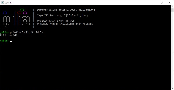
REPL (read-eval-print loop) is the working environment of Julia. With the help of this shell we can interact with Julias JIT (Just in Time) compiler to test and run our code. We can also copy and paste our code into .jl extension, for example, first.jl. Another option is to use a text editor or IDE. Let us have a look at REPL below −
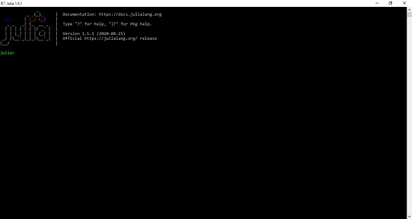
After clicking on Julia logo, we will get a prompt with julia> for writing our piece of code or program. Use exit() or CTRL + D to end the session. If you want to evaluate the expression, press enter after input.

Packages
Almost all the standard libraries in Julia are written in Julia itself but the rest of the Julias code ecosystem can be found in Packages which are Git repositories. Some important points about Julia packages are given below −
Packages provide reusable functionality that can be easily used by other Julia projects.
Julia has built-in package manager named pkg.jl for package installation.
The package manager handles installation, removal, and updates of packages.
The package manager works only if the packages are in REPL.
Installing packages
Step 1 − First open the Julia command line.

Step 2 − Now open the Julia package management environment by pressing, ]. You will get the following console −

You can check https://discourse.julialang.org/t/shutting-down-julia-observer-posted-4-1-20/36870 to see which packages we can install on Julia.
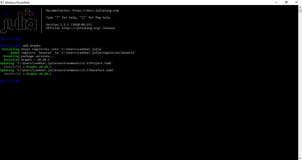
Adding a package
For adding a package in Julia environment, we need to use addcommand with the name of the package. For example, we will be adding the package named Graphs which is uses for working with graphs in Julia.
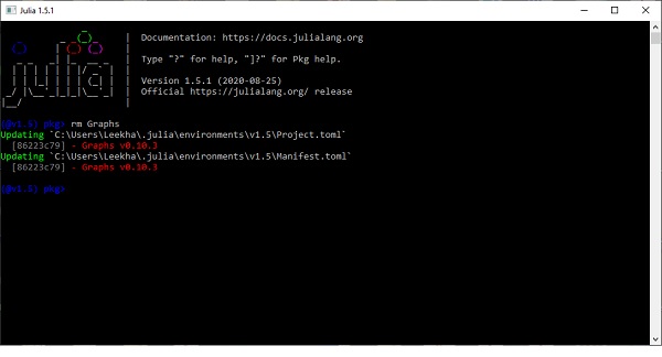
Removing a package
For removing a package from Julia, we need to use rm command with the name of the of the package. For example, we will be removing the package named Graphs as follows −
Updating a package
To update a Julia package, either you can use update command, which will update all the Julia packages, or you can use up command along with the name of the package, which will update specific package.
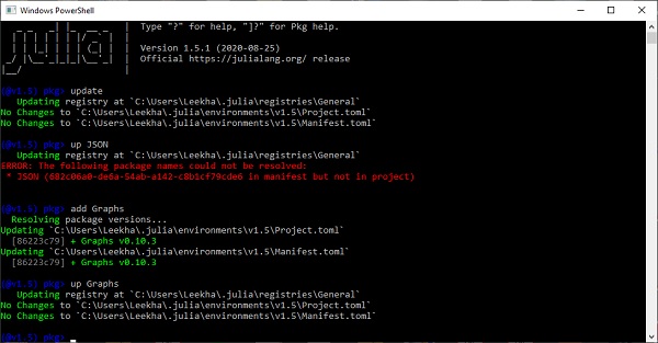
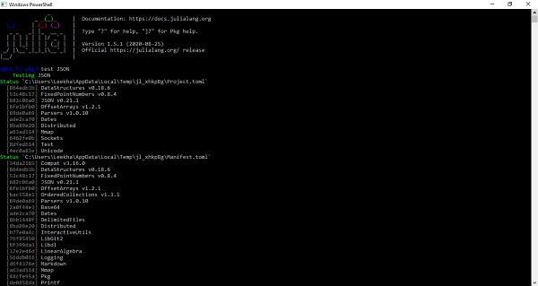
Testing a package
Use test command to test a Julia package. For example, below we have tested JSON package −
Installing IJulia
To install IJulia, use add IJulia command in Julia package environment. We need to make sure that you have preinstalled Anaconda on your machine. Once it gets installed, open Jupyter notebook and choose Julia1.5.1 as follows −
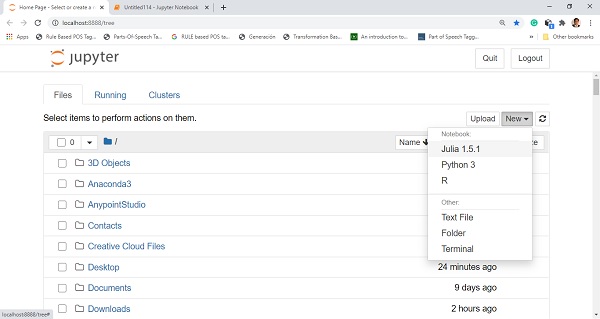
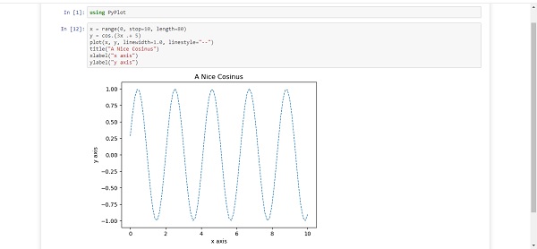
Now you will be able to write Julia programs using IJulia as follows −
Installing Juno
Juno is a powerful IDE for Julia programming language. It is free, and to install follow the steps given below −
Step 1 − First we need to install Julia on our system.
Step 2 − Now you need to install Atom from here. It must be updated(version 1.41+).
Step 3 − In Atom, go to settings and then install panel. It will install Juno for you.
Step 4 − Start working in Juno by opening REPL with Juno > open REPL command.
Julia Programming - Basic Syntax
The simplest first Julia program (and of many other programming languages too) is to print hello world. The script is as follows −
If you have added Julia to your path, the same script can be saved in a file say hello.jl and can be run by typing Julia hello.jl at command prompt. Alternatively the same can also be run from Julia REPL by typing include(hello.jl). This command will evaluate all valid expressions and return the last output.
Variables
What can be the simplest definition of a computer program? The simplest one may be that a computer program is a series of instructions to be executed on a variety of data.
Here the data can be the name of a person, place, the house number of a person, or even a list of things you have made. In computer programming, when we need to label such information, we give it a name (say A) and call it a variable. In this sense, we can say that a variable is a box containing data.
Let us see how we can assign data to a variable. It is quite simple, just type it. For example,
student_name = Ramroll_no = 15marks_math = 9.5
Here, the first variable i.e. student_name contains a string, the second variable i.e. roll_no contains a number, and the third variable i.e. marks_math contains a floating-point number. We see, unlike other programming languages such as C++, Python, etc.,in Julia we do not have to specify the type of variables because it can infer the type of object on the right side of the equal sign.
Stylistic Conventions and Allowed Variable Names
Following are some conventions used for variables names −
The names of the variables in Julia are case sensitive. So, the variables student_name and Student_name would not be same.
The names of the variables in Julia should always start with a letter and after that we can use anything like digits, letters, underscores, etc.
In Julia, generally lower-case letter is used with multiple words separated by an underscore.
We should use clear, short, and to the point names for variables.
Some of the valid Julia variable names are student_name, roll_no, speed, current_time.
Comments
Writing comments in Julia is quite same as Python. Based on the usage, comments are of two types −
Single Line Comments
In Julia, the single line comments start with the symbol of # (hashtag) and it lasts till the end of that line. Suppose if your comment exceeds one line then you should put a # symbol on the next line also and can continue the comment. Given below is the code snippet showing single line comment −
Example
julia> #This is an example to demonstrate the single lined comments.julia> #Print the given name
Multi-line Comments
In Julia, the multi-line comment is a piece of text, like single line comment, but it is enclosed in a delimiter #= on the start of the comment and enclosed in a delimiter =# on the end of the comment. Given below is the code snippet showing multi-line comment −
Example
julia> #= This is an example to demonstrate the multi-line comments that tells us about tutorialspoint.com. At this website you can browse the best resource for Online Education.=#julia> print(www.tutorialspoint.com)
Julia - Arrays
An Array is an ordered set of elements which are often specified with squared brackets having comma-separated items. We can create arrays that are −
Full or empty
Hold values of different types
Restricted to values of a specific type
In Julia, arrays are actually mutable type collections which are used for lists, vectors, tables, and matrices. That is why the values of arrays in Julia can be modified with the use of certain pre-defined keywords. With the help of push! command you can add new element in array. Similarly, with the help of splice! function you can add elements in an array at a specified index.
Creating Simple 1D Arrays
Following is the example showing how we can create a simple 1D array −
julia> arr = [1,2,3]3-element Array{Int64,1}: 1 2 3The above example shows that we have created a 1D array with 3 elements each of which is a 64-bit integer. This 1D array is bound to the variable arr.
Uninitialized array
We can also specify the type and the dimension of an array by using the below syntax −
Array{type}(dims)Following is an example of uninitialized array −
julia> array = Array{Int64}(undef, 3)3-element Array{Int64,1}: 0 0 0julia> array = Array{Int64}(undef, 3, 3, 3)333 Array{Int64,3}:[:, :, 1] = 8 372354944 328904752 3 331059280 162819664 32 339708912 1 [:, :, 2] = 331213072 3 331355760 1 328841776 331355984 -1 328841680 2[:, :, 3] = 1 0 339709232 164231472 328841872 347296224 328841968 339709152 16842753Here we placed the type in curly braces and the dimensions in parentheses. We use undef which means that particular array has not been initialized to any known value and thats why we got random numbers in the output.
Arrays of anything
Julia gives us the freedom to create arrays with elements of different types. Let us see the example below in which we are going to create array of an odd mixture numbers, strings, functions, constants −
julia> [1, "TutorialsPoint.com", 5.5, tan, pi]5-element Array{Any,1}: 1 "TutorialsPoint.com" 5.5 tan (generic function with 12 methods) = 3.1415926535897...Empty Arrays
Just like creating an array of specific type, we can also create empty arrays in Julia. The example is given below −
julia> A = Int64[]Int64[]julia> A = String[]String[]
Creating 2D arrays & matrices
Leave out the comma between elements and you will be getting 2D arrays in Julia. Below is the example given for single row, multi-column array −
julia> [1 2 3 4 5 6 7 8 9 10]110 Array{Int64,2}: 1 2 3 4 5 6 7 8 9 10Here, 110 is the first row of this array.
To add another row, just add a semicolon(;). Let us check the below example −
julia> [1 2 3 4 5 ; 6 7 8 9 10]25 Array{Int64,2}: 1 2 3 4 5 6 7 8 9 10Here, it becomes 25 array.
Creating arrays using range objects
We can create arrays using range objects in the following ways −
Collect() function
First useful function to create an array using range objects is collect(). With the help of colon(:) and collect() function, we can create an array using range objects as follows −
julia> collect(1:5)5-element Array{Int64,1}: 1 2 3 4 5We can also create arrays with floating point range objects −
julia> collect(1.5:5.5)5-element Array{Float64,1}: 1.5 2.5 3.5 4.5 5.5Let us see a three-piece version of a range object with the help of which you can specify a step size other than 1.
The syntax for the same is given below −start:step:stop.
Below is an example to build an array with elements that go from 0 to 50 in steps of 5 −
julia> collect(0:5:50)11-element Array{Int64,1}: 0 5 10 15 20 25 30 35 40 45 50 ellipsis() or splat operator
Instead of using collect() function, we can also use splat operator or ellipsis() after the last element. Following is an example −
julia> [0:10...]11-element Array{Int64,1}: 0 1 2 3 4 5 6 7 8 9 10range() function
Range() is another useful function to create an array with range objects. It goes from start value to end value by taking a specific step value.
For example, let us see an example to go from 1 to 150 in exactly 15 steps −
julia> range(1, length=15, stop=150)1.0:10.642857142857142:150.0Or you can use range to take 10 steps from 1, stopping at or before 150:julia> range(1, stop=150, step=10)1:10:141
We can use range() with collect() to build an array as follows −
julia> collect(range(1, length=15, stop=150))15-element Array{Float64,1}: 1.0 11.642857142857142 22.285714285714285 32.92857142857143 43.57142857142857 54.214285714285715 64.85714285714286 75.5 86.14285714285714 96.78571428571429 107.42857142857143 118.07142857142857 128.71428571428572 139.35714285714286 150.0Creating arrays using comprehensions and generators
Another useful way to create an array is to use comprehensions. In this way, we can create array where each element can produce using a small computation. For example, we can create an array of 10 elements as follows −
julia> [n^2 for n in 1:10]10-element Array{Int64,1}: 1 4 9 16 25 36 49 64 81 100We can easily create a 2-D array also as follows −
julia> [n*m for n in 1:10, m in 1:10]1010 Array{Int64,2}: 1 2 3 4 5 6 7 8 9 10 2 4 6 8 10 12 14 16 18 20 3 6 9 12 15 18 21 24 27 30 4 8 12 16 20 24 28 32 36 40 5 10 15 20 25 30 35 40 45 50 6 12 18 24 30 36 42 48 54 60 7 14 21 28 35 42 49 56 63 70 8 16 24 32 40 48 56 64 72 80 9 18 27 36 45 54 63 72 81 90 10 20 30 40 50 60 70 80 90 100Similar to comprehension, we can use generator expressions to create an array −
julia> collect(n^2 for n in 1:5)5-element Array{Int64,1}: 1 4 9 16 25Generator expressions do not build an array to first hold the values rather they generate the values when needed. Hence they are more useful than comprehensions.
Populating an Array
Following are the functions with the help of which you can create and fill arrays with specific contents −
zeros (m, n)
This function will create matrix of zeros with m number of rows and n number of columns. The example is given below −
julia> zeros(4,5)45 Array{Float64,2}: 0.0 0.0 0.0 0.0 0.0 0.0 0.0 0.0 0.0 0.0 0.0 0.0 0.0 0.0 0.0 0.0 0.0 0.0 0.0 0.0We can also specify the type of zeros as follows −
julia> zeros(Int64,4,5)45 Array{Int64,2}: 0 0 0 0 0 0 0 0 0 0 0 0 0 0 0 0 0 0 0ones (m, n)
This function will create matrix of ones with m number of rows and n number of columns. The example is given below −
julia> ones(4,5)45 Array{Float64,2}: 1.0 1.0 1.0 1.0 1.0 1.0 1.0 1.0 1.0 1.0 1.0 1.0 1.0 1.0 1.0 1.0 1.0 1.0 1.0 1.0rand (m, n)
As the name suggests, this function will create matrix of random numbers with m number of rows and n number of columns. The example is given below −
julia> rand(4,5)45 Array{Float64,2}: 0.514061 0.888862 0.197132 0.721092 0.899983 0.503034 0.81519 0.061025 0.279143 0.204272 0.687983 0.883176 0.653474 0.659005 0.970319 0.20116 0.349378 0.470409 0.000273225 0.83694randn(m, n)
As the name suggests, this function will create m*n matrix of normally distributed random numbers with mean=0 and standard deviation(SD)=1.
julia> randn(4,5)45 Array{Float64,2}: -0.190909 -1.18673 2.17422 0.811674 1.32414 0.837096 -0.0326669 -2.03179 0.100863 0.409234 -1.24511 -0.917098 -0.995239 0.820814 1.60817 -1.00931 -0.804208 0.343079 0.0771786 0.361685fill()
This function is used to fill an array with a specific value. More specifically, it will create an array of repeating duplicate value.
julia> fill(100,5)5-element Array{Int64,1}: 100 100 100 100 100 julia> fill("tutorialspoint.com",3,3)33 Array{String,2}:"tutorialspoint.com" "tutorialspoint.com" "tutorialspoint.com""tutorialspoint.com" "tutorialspoint.com" "tutorialspoint.com""tutorialspoint.com" "tutorialspoint.com" "tutorialspoint.com"fill!()
It is similar to fill() function but the sign of exclamation (!) is an indication or warning that the content of an existing array is going to be changed. The example is given below:
julia> ABC = ones(5)5-element Array{Float64,1}: 1.0 1.0 1.0 1.0 1.0 julia> fill!(ABC,100)5-element Array{Float64,1}: 100.0 100.0 100.0 100.0 100.0 julia> ABC5-element Array{Float64,1}: 100.0 100.0 100.0 100.0 100.0Array Constructor
The function Array(), we have studied earlier, can build array of a specific type as follows −
julia> Array{Int64}(undef, 5)5-element Array{Int64,1}: 294967297 8589934593 8589934594 8589934594 0As we can see from the output that this array is uninitialized. The odd-looking numbers are memories old content.
Arrays of arrays
Following example demonstrates creating arrays of arrays −
julia> ABC = Array[[3,4],[5,6]]2-element Array{Array,1}: [3, 4] [5, 6]It can also be created with the help of Array constructor as follows −
julia> Array[1:5,6:10]2-element Array{Array,1}: [1, 2, 3, 4, 5] [6, 7, 8, 9, 10]Copying arrays
Suppose you have an array and want to create another array with similar dimensions, then you can use similar() function as follows −
julia> A = collect(1:5);Here we have hide the values with the help of semicolon(;)julia> B = similar(A)5-element Array{Int64,1}: 164998448 234899984 383606096 164557488 396984416Here the dimension of array A are copied but not values.
Matrix Operations
As we know that a two-dimensional (2D) array can be used as a matrix so all the functions that are available for working on arrays can also be used as matrices. The condition is that the dimensions and contents should permit. If you want to type a matrix, use spaces to make rows and semicolon(;) to separate the rows as follows −
julia> [2 3 ; 4 5]22 Array{Int64,2}: 2 3 4 5Following is an example to create an array of arrays (as we did earlier) by placing two arrays next to each other −
julia> Array[[3,4],[5,6]]2-element Array{Array,1}: [3, 4] [5, 6]Below we can see what happens when we omit the comma and place columns next to each other −
julia> [[3,4] [5,6]]22 Array{Int64,2}: 3 5 4 6Accessing the contents of arrays
In Julia, to access the contents/particular element of an array, you need to write the name of the array with the element number in square bracket.
Below is an example of 1-D array −
julia> arr = [5,10,15,20,25,30,35,40,45,50]10-element Array{Int64,1}: 5 10 15 20 25 30 35 40 45 50julia> arr[4]20In some programming languages, the last element of an array is referred to as -1. However, in Julia, it is referred to as end. You can find the last element of an array as follows −
julia> arr[end]50
And the second last element as follows −
julia> arr[end-1]45
To access more than one element at a time, we can also provide a bunch of index numbers as shown below −
julia> arr[[2,5,6]]3-element Array{Int64,1}: 10 25 30We can access array elements even by providing true and false −
julia> arr[[true, false, true, true,true, false, false, true, true, false]]6-element Array{Int64,1}: 5 15 20 25 40 45Now let us access the elements of 2-D.
julia> arr2 = [10 11 12; 13 14 15; 16 17 18]33 Array{Int64,2}: 10 11 12 13 14 15 16 17 18julia> arr2[1]10The below command will give 13 not 11 as we were expecting.
julia> arr2[2]13
To access row1, column2 element, we need to use the command below −
julia> arr2[1,2]11
Similarly, for row1 and column3 element, we have to use the below command −
julia> arr2[1,3]12
We can also use getindex() function to obtain elements from a 2-D array −
julia> getindex(arr2,1,2)11julia> getindex(arr2,2,3)15
Adding Elements
We can add elements to an array in Julia at the end, at the front and at the given index using push!(), pushfirst!() and splice!() functions respectively.
At the end
We can use push!() function to add an element at the end of an array. For example,
julia> push!(arr,55)11-element Array{Int64,1}: 5 10 15 20 25 30 35 40 45 50 55Remember we had 10 elements in array arr. Now push!() function added the element 55 at the end of this array.
The exclamation(!) sign represents that the function is going to change the array.
At the front
We can use pushfirst!() function to add an element at the front of an array. For example,
julia> pushfirst!(arr,0)12-element Array{Int64,1}: 0 5 10 15 20 25 30 35 40 45 50 55At a given index
We can use splice!() function to add an element into an array at a given index. For example,
julia> splice!(arr,2:5,2:6)4-element Array{Int64,1}: 5 10 15 20julia> arr13-element Array{Int64,1}: 0 2 3 4 5 6 25 30 35 40 45 50 55Removing Elements
We can remove elements at last position, first position and at the given index, from an array in Julia, using pop!(), popfirst!() and splice!() functions respectively.
Remove the last element
We can use pop!() function to remove the last element of an array. For example,
julia> pop!(arr)55julia> arr12-element Array{Int64,1}: 0 2 3 4 5 6 25 30 35 40 45 50Removing the first element
We can use popfirst!() function to remove the first element of an array. For example,
julia> popfirst!(arr)0julia> arr11-element Array{Int64,1}: 2 3 4 5 6 25 30 35 40 45 50Removing element at given position
We can use splice!() function to remove the element from a given position of an array. For example,
julia> splice!(arr,5)6julia> arr10-element Array{Int64,1}: 2 3 4 5 25 30 35 40 45 50Julia - Tuples
Similar to an array, tuple is also an ordered set of elements. Tuples work in almost the same way as arrays but there are following important differences between them −
An array is represented by square brackets whereas a tuple is represented by parentheses and commas.
Tuples are immutable.
Creating tuples
We can create tuples as arrays and most of the arrays functions can be used on tuples also. Some of the example are given below −
julia> tupl=(5,10,15,20,25,30)(5, 10, 15, 20, 25, 30)julia> tupl(5, 10, 15, 20, 25, 30)julia> tupl[3:end](15, 20, 25, 30)julia> tupl = ((1,2),(3,4))((1, 2), (3, 4))julia> tupl[1](1, 2)julia> tupl[1][2]2We cannot change a tuple:julia> tupl[2]=0ERROR: MethodError: no method matching setindex!(::Tuple{Tuple{Int64,Int64},Tuple{Int64,Int64}}, ::Int64, ::Int64)Stacktrace: [1] top-level scope at REPL[7]:1Named tuples
A named tuple is simply a combination of a tuple and a dictionary because −
A named tuple is ordered and immutable like a tuple and
Like a dictionary in named tuple, each element has a unique key which can be used to access it.
In next section, let us see how we can create named tuples −
Creating named tuples
You can create named tuples in Julia by −
Providing keys and values in separate tuples
Providing keys and values in a single tuple
Combining two existing named tuples
Keys and values in separate tuples
One way to create named tuples is by providing keys and values in separate tuples.
Example
julia> names_shape = (:corner1, :corner2)(:corner1, :corner2)julia> values_shape = ((100, 100), (200, 200))((100, 100), (200, 200))julia> shape_item2 = NamedTuple{names_shape}(values_shape)(corner1 = (100, 100), corner2 = (200, 200))We can access the elements by using dot(.) syntax −
julia> shape_item2.corner1(100, 100)julia> shape_item2.corner2(200, 200)
Keys and values in a single tuple
We can also create named tuples by providing keys and values in a single tuple.
Example
julia> shape_item = (corner1 = (1, 1), corner2 = (-1, -1), center = (0, 0))(corner1 = (1, 1), corner2 = (-1, -1), center = (0, 0))
We can access the elements by using dot(.) syntax −
julia> shape_item.corner1(1, 1)julia> shape_item.corner2(-1, -1)julia> shape_item.center(0, 0)julia> (shape_item.center,shape_item.corner2)((0, 0), (-1, -1))
We can also access all the values as with ordinary tuples as follows −
julia> c1, c2, center = shape_item(corner1 = (1, 1), corner2 = (-1, -1), center = (0, 0))julia> c1(1, 1)
Combining two named tuples
Julia provides us a way to make new named tuples by combining two named tuples together as follows −
Example
julia> colors_shape = (top = "red", bottom = "green")(top = "red", bottom = "green")julia> shape_item = (corner1 = (1, 1), corner2 = (-1, -1), center = (0, 0))(corner1 = (1, 1), corner2 = (-1, -1), center = (0, 0))julia> merge(shape_item, colors_shape)(corner1 = (1, 1), corner2 = (-1, -1), center = (0, 0), top = "red", bottom = "green")
Named tuples as keyword arguments
If you want to pass a group of keyword arguments to a function, named tuple is a convenient way to do so in Julia. Following is the example of a function that accepts three keyword arguments −
julia> function ABC(x, y, z; a=10, b=20, c=30) println("x = $x, y = $y, z = $z; a = $a, b = $b, c = $c") endABC (generic function with 1 method)It is also possible to define a named tuple which contains the names as well values for one or more keywords as follows −
julia> options = (b = 200, c = 300)(b = 200, c = 300)
In order to pass the named tuples to the function we need to use; while calling the function −
julia> ABC(1, 2, 3; options...)x = 1, y = 2, z = 3; a = 10, b = 200, c = 300
The values and keyword can also be overridden by later function as follows −
julia> ABC(1, 2, 3; b = 1000_000, options...)x = 1, y = 2, z = 3; a = 10, b = 200, c = 300julia> ABC(1, 2, 3; options..., b= 1000_000)x = 1, y = 2, z = 3; a = 10, b = 1000000, c = 300
Integers and Floating-Point Numbers
In any programming language, there are two basic building blocks of arithmetic and computation. They are integers and floating-point values. Built-in representation of the values of integers and floating-point are called numeric primitives. On the other hand, their representation as immediate values in code are called numeric literals.
Following are the example of integer and floating-point literals −
100 is an integer literal
100.50 is a floating-point literal
Their built-in memory representations as objects is numeric primitives.
Integers
Integer is one of the primitive numeric types in Julia. It is represented as follows −
julia> 100100julia> 123456789123456789
We can check the default type of an integer literal, which depends on whether our system is 32-bit or 64-bit architecture.
julia> Sys.WORD_SIZE64julia> typeof(100)Int64
Integer types
The table given below shows the integer types in Julia −
| Type | Signed? | Number of bits | Smallest value | Largest value |
|---|---|---|---|---|
| Int8 | ✓ | 8 | -2^7 | 2^7 1 |
| UInt8 | 8 | 0 | 2^8 1 | |
| Int16 | ✓ | 16 | -2^15 | 2^15 1 |
| UInt16 | 16 | 0 | 2^16 1 | |
| Int32 | ✓ | 32 | -2^31 | 2^31 1 |
| UInt32 | 32 | 0 | 2^32 1 | |
| Int64 | ✓ | 64 | -2^63 | 2^63 1 |
| UInt64 | 64 | 0 | 2^64 1 | |
| Int128 | ✓ | 128 | -2^127 | 2^127 1 |
| UInt128 | 128 | 0 | 2^128 1 | |
| Bool | N/A | 8 | false (0) | true (1) |
Overflow behavior
In Julia, if the maximum representable value of a given type exceeds, then it results in a wraparound behavior. For example −
julia> A = typemax(Int64)9223372036854775807julia> A + 1-9223372036854775808julia> A + 1 == typemin(Int64)true
It is recommended to explicitly check for wraparound produced by overflow especially where overflow is possible. Otherwise use BigInt type in Arbitrary Precision Arithmetic.
Below is an example of overflow behavior and how we can resolve it −
julia> 10^19-8446744073709551616julia> big(10)^1910000000000000000000
Division errors
Integer division throws a DivideError in the following two exceptional cases −
Dividing by zero
Dividing the lowest negative number
The rem (remainder) and mod (modulus) functions will throw a DivideError whenever their second argument is zero. The example are given below −
julia> mod(1, 0)ERROR: DivideError: integer division errorStacktrace: [1] div at .\int.jl:260 [inlined] [2] div at .\div.jl:217 [inlined] [3] div at .\div.jl:262 [inlined] [4] fld at .\div.jl:228 [inlined] [5] mod(::Int64, ::Int64) at .\int.jl:252 [6] top-level scope at REPL[52]:1 julia> rem(1, 0)ERROR: DivideError: integer division errorStacktrace: [1] rem(::Int64, ::Int64) at .\int.jl:261 [2] top-level scope at REPL[54]:1
Floating-point numbers
Another primitive numeric types in Julia is floating-point numbers. It is represented (using E-notation when needed) as follows −
julia> 1.01.0julia> 0.50.5julia> -1.256-1.256julia> 2e112.0e11julia> 3.6e-53.6e-5
All the above results are Float64. If we would like to enter Float32 literal, they can be written by writing f in the place of e as follows −
julia> 0.5f-55.0f-6julia> typeof(ans)Float32julia> 1.5f01.5f0julia> typeof(ans)Float32
Floating-point types
The table given below shows the floating-point types in Julia −
Floating-point zeros
There are two kind of floating-point zeros, one is positive zero and other is negative zero. They are same but their binary representation is different. It can be seen in the example below −
julia> 0.0 == -0.0truejulia> bitstring(0.0)"0000000000000000000000000000000000000000000000000000000000000000"julia> bitstring(-0.0)"1000000000000000000000000000000000000000000000000000000000000000"
Special floating-point values
The table below represents three specified standard floating-point values. These floating-point values do not correspond to any point on the real number line.
| Float16 | Float32 | Float64 | Name | Description |
|---|---|---|---|---|
| Inf16 | Inf32 | Inf | positive infinity | It is the value greater than all finite floating-point values |
| -Inf16 | -Inf32 | -Inf | negative infinity | It is the value less than all finite floating-point values |
| NaN16 | NaN32 | NaN | not a number | It is a value not == to any floating-point value (including itself) |
We can also apply typemin and typemax functions as follows −
julia> (typemin(Float16),typemax(Float16))(-Inf16, Inf16)julia> (typemin(Float32),typemax(Float32))(-Inf32, Inf32)julia> (typemin(Float64),typemax(Float64))(-Inf, Inf)
Machine epsilon
Machine epsilon is the distance between two adjacent representable floating-point numbers. It is important to know machine epsilon because most of the real numbers cannot be represented exactly with floating-point numbers.
In Julia, we have eps() function that gives us the distance between 1.0 and the next larger representable floating-point value. The example is given below −
julia> eps(Float32)1.1920929f-7julia> eps(Float64)2.220446049250313e-16
Rounding modes
As we know that the number should be rounded to an appropriate representable value if it does not have an exact floating-point representation. Julia uses the default mode called RoundNearest. It rounds to the nearest integer, with ties being rounded to the nearest even integer. For example,
julia> BigFloat("1.510564889",2,RoundNearest)1.5Rational and Complex Numbers
In this chapter, we shall discuss rational and complex numbers.
Rational Numbers
Julia represents exact ratios of integers with the help of rational number type. Let us understand about rational numbers in Julia in further sections −
Constructing rational numbers
In Julia REPL, the rational numbers are constructed by using the operator //. Below given is the example for the same −
julia> 4//54//5
You can also extract the standardized numerator and denominator as follows −
julia> numerator(8//9)8julia> denominator(8//9)9
Converting to floating-point numbers
It is very easy to convert the rational numbers to floating-point numbers. Check out the following example −
julia> float(2//3)0.6666666666666666Converting rational to floating-point numbers does not loose the following identity for any integral values of A and B. For example:julia> A = 20; B = 30;julia> isequal(float(A//B), A/B)true
Complex Numbers
As we know that the global constant im, which represents the principal square root of -1, is bound to the complex number. This binding in Julia suffice to provide convenient syntax for complex numbers because Julia allows numeric literals to be contrasted with identifiers as coefficients.
julia> 2+3im2 + 3im
Performing Standard arithmetic operations
We can perform all the standard arithmetic operations on complex numbers. The example are given below −
julia> (2 + 3im)*(1 - 2im)8 - 1imjulia> (2 + 3im)/(1 - 2im)-0.8 + 1.4imjulia> (2 + 3im)+(1 - 2im)3 + 1imjulia> (2 + 3im)-(1 - 2im)1 + 5imjulia> (2 + 3im)^2-5 + 12imjulia> (2 + 3im)^2.6-23.375430842463754 + 15.527174176755075imjulia> 2(2 + 3im)4 + 6imjulia> 2(2 + 3im)^-2.0-0.059171597633136105 - 0.14201183431952663im
Combining different operands
The promotion mechanism in Julia ensures that combining different kind of operators works fine on complex numbers. Let us understand it with the help of the following example −
julia> 2(2 + 3im)4 + 6imjulia> (2 + 3im)-11 + 3imjulia> (2 + 3im)+0.72.7 + 3.0imjulia> (2 + 3im)-0.7im2.0 + 2.3imjulia> 0.89(2 + 3im)1.78 + 2.67imjulia> (2 + 3im)/21.0 + 1.5imjulia> (2 + 3im)/(1-3im)-0.7000000000000001 + 0.8999999999999999imjulia> 3im^30 - 3imjulia> 1+2/5im1.0 - 0.4im
Functions to manipulate complex values
In Julia, we can also manipulate the values of complex numbers with the help of standard functions. Below are given some example for the same −
julia> real(4+7im) #real part of complex number4julia> imag(4+7im) #imaginary part of complex number7julia> conj(4+7im) # conjugate of complex number4 - 7imjulia> abs(4+7im) # absolute value of complex number8.06225774829855julia> abs2(4+7im) #squared absolute value65julia> angle(4+7im) #phase angle in radians1.0516502125483738
Let us check out the use of Elementary Functions for complex numbers in the below example −
julia> sqrt(7im) #square root of imaginary part1.8708286933869707 + 1.8708286933869707imjulia> sqrt(4+7im) #square root of complex number2.455835677350843 + 1.4251767869809258imjulia> cos(4+7im) #cosine of complex number-358.40393224005317 + 414.96701031076253imjulia> exp(4+7im) #exponential of complex number41.16166839296141 + 35.87025288661357imjulia> sinh(4+7im) #Hyperbolic sine value of complex number20.573930095756726 + 17.941143007955223im
Julia - Basic Operators
In this chapter, we shall discuss different types of operators in Julia.
Arithmetic Operators
In Julia, we get all the basic arithmetic operators across all the numeric primitive types. It also provides us bitwise operators as well as efficient implementation of comprehensive collection of standard mathematical functions.
Following table shows the basic arithmetic operators that are supported on Julias primitive numeric types −
| Expression | Name | Description |
|---|---|---|
| +x | unary plus | It is the identity operation. |
| -x | unary minus | It maps values to their additive inverses. |
| x + y | binary plus | It performs addition. |
| x - y | binary minus | It performs subtraction. |
| x * y | times | It performs multiplication. |
| x / y | divide | It performs division. |
| x y | integer divide | Denoted as x / y and truncated to an integer. |
| x \ y | inverse divide | It is equivalent to y / x. |
| x ^ y | power | It raises x to the yth power. |
| x % y | remainder | It is equivalent to rem(x,y). |
| !x | negation | It is negation on bool types and changes true to false and vice versa. |
The promotion system of Julia makes these arithmetic operations work naturally and automatically on the mixture of argument types.
Example
Following example shows the use of arithmetic operators −
julia> 2+20-517julia> 3-8-5julia> 50*2/1010.0julia> 23%21julia> 2^416
Bitwise Operators
Following table shows the bitwise operators that are supported on Julias primitive numeric types −
| Sl.No | Expression Name | Name |
|---|---|---|
| 1 | ∼x | bitwise not |
| 2 | x & y | bitwise and |
| 3 | x | y | bitwise or |
| 4 | x ⊻ y | bitwise xor (exclusive or) |
| 5 | x >>> y | logical shift right |
| 6 | x >> y | arithmetic shift right |
| 7 | x << y | logical/arithmetic shift left |
Example
Following example shows the use of bitwise operators −
julia> ∼1009-1010julia> 12&234julia> 12 & 234julia> 12 | 2331julia> 12 ⊻ 2327julia> xor(12, 23)27julia> ∼UInt32(12)0xfffffff3julia> ∼UInt8(12)0xf3
Updating Operators
Each arithmetic as well as bitwise operator has an updating version which can be formed by placing an equal sign (=) immediately after the operator. This updating operator assigns the result of the operation back into its left operand. It means that a +=1 is equal to a = a+1.
Following is the list of the updating versions of all the binary arithmetic and bitwise operators −
+=
-=
*=
/=
\=
÷=
%=
^=
&=
|=
⊻=
>>>=
>>=
<<=
Example
Following example shows the use of updating operators −
julia> A = 100100julia> A +=100200julia> A200
Vectorized dot Operators
For each binary operation like ^, there is a corresponding dot(.) operation which is used on the entire array, one by one. For instance, if you would try to perform [1, 2, 3] ^ 2, then it is not defined and not possible to square an array. On the other hand, [1, 2, 3] .^ 2 is defined as computing the vectorized result. In the same sense, this vectorized dot operator can also be used with other binary operators.
Example
Following example shows the use of dot operator −
julia> [1, 2, 3].^23-element Array{Int64,1}: 1 4 9Numeric Comparisons Operators
Following table shows the numeric comparison operators that are supported on Julias primitive numeric types −
| Sl.No | Operator | Name |
|---|---|---|
| 1 | == | Equality |
| 2 | !=,≠ | inequality |
| 3 | < | less than |
| 4 | <=, ≤ | less than or equal to |
| 5 | > | greater than |
| 6 | >=, ≥ | greater than or equal to |
Example
Following example shows the use of numeric comparison operators −
julia> 100 == 100truejulia> 100 == 101falsejulia> 100 != 101truejulia> 100 == 100.0truejulia> 100 < 500truejulia> 100 > 500falsejulia> 100 >= 100.0truejulia> -100 <= 100truejulia> -100 <= -100truejulia> -100 <= -500falsejulia> 100 < -10.0false
Chaining Comparisons
In Julia, the comparisons can be arbitrarily chained. In case of numerical code, the chaining comparisons are quite convenient. The && operator for scalar comparisons and & operator for elementwise comparison allows chained comparisons to work fine on arrays.
Example
Following example shows the use of chained comparison −
julia> 100 < 200 <= 200 < 300 == 300 > 200 >= 100 == 100 < 300 != 500true
In the following example, let us check out the evaluation behavior of chained comparisons −
julia> M(a) = (println(a); a)M (generic function with 1 method)julia> M(1) < M(2) <= M(3) 2 1 3truejulia> M(1) > M(2) <= M(3) 2 1false
Operator Precedence & Associativity
From highest precedence to lowest, the following table shows the order and associativity of operations applied by Julia −
| Category | Operators | Associativity |
|---|---|---|
| Syntax | followed by :: | Left |
| Exponentiation | ^ | Right |
| Unary | + - | Right |
| Bitshifts | << >> >>> | Left |
| Fractions | // | Left |
| Multiplication | * / % & \ ÷ | Left |
| Addition | + - | ⊻ | Left |
| Syntax | : .. | Left |
| Syntax | |> | Left |
| Syntax | <| | Right |
| Comparisons | > < >= <= == === != !== <: | Non-associative |
| Control flow | && followed by || followed by ? | Right |
| Pair | => | Right |
| Assignments | = += -= *= /= //= \= ^= = %= |= &= ⊻= <<= >>= >>>= | Right |
We can also use Base.operator_precedence function to check the numerical precedence of a given operator. The example is given below −
julia> Base.operator_precedence(:-), Base.operator_precedence(:+), Base.operator_precedence(:.)(11, 11, 17)
Basic Mathematical Functions
Let us try to understand basic mathematical functions with the help of example in this chapter.
Numerical Conversions
In Julia, the user gets three different forms of numerical conversion. All the three differ in their handling of inexact conversions. They are as follows −
T(x) or convert(T, x) − This notation converts x to a value of T. The result depends upon following two cases −
T is a floating-point type − In this case the result will be the nearest representable value. This value could be positive or negative infinity.
T is an integer type − The result will raise an InexactError if and only if x is not representable by T.
x%T − This notation will convert an integer x to a value of integer type T corresponding to x modulo 2^n. Here n represents the number of bits in T. In simple words, this notation truncates the binary representation to fit.
Rounding functions − This notation takes a type T as an optional argument for calculation. Eg − Round(Int, a) is shorthand for Int(round(a)).
Example
The example given below represent the various forms described above −
julia> Int8(110)110julia> Int8(128)ERROR: InexactError: trunc(Int8, 128)Stacktrace: [1] throw_inexacterror(::Symbol, ::Type{Int8}, ::Int64) at .\boot.jl:558 [2] checked_trunc_sint at .\boot.jl:580 [inlined] [3] toInt8 at .\boot.jl:595 [inlined] [4] Int8(::Int64) at .\boot.jl:705 [5] top-level scope at REPL[4]:1 julia> Int8(110.0)110julia> Int8(3.14)ERROR: InexactError: Int8(3.14)Stacktrace: [1] Int8(::Float64) at .\float.jl:689 [2] top-level scope at REPL[6]:1julia> Int8(128.0)ERROR: InexactError: Int8(128.0)Stacktrace: [1] Int8(::Float64) at .\float.jl:689 [2] top-level scope at REPL[7]:1julia> 110%Int8110julia> 128%Int8-128julia> round(Int8, 110.35)110julia> round(Int8, 127.52)ERROR: InexactError: trunc(Int8, 128.0)Stacktrace: [1] trunc at .\float.jl:682 [inlined] [2] round(::Type{Int8}, ::Float64) at .\float.jl:367 [3] top-level scope at REPL[14]:1Rounding functions
Following table shows rounding functions that are supported on Julias primitive numeric types −
| Function | Description | Return type |
|---|---|---|
| round(x) | This function will round x to the nearest integer. | typeof(x) |
| round(T, x) | This function will round x to the nearest integer. | T |
| floor(x) | This function will round x towards -Inf returns the nearest integral value of the same type as x. This value will be less than or equal to x. | typeof(x) |
| floor(T, x) | This function will round x towards -Inf and converts the result to type T. It will throw an InexactError if the value is not representable. | T |
| floor(T, x) | This function will round x towards -Inf and converts the result to type T. It will throw an InexactError if the value is not representable. | T |
| ceil(x) | This function will round x towards +Inf and returns the nearest integral value of the same type as x. This value will be greater than or equal to x. | typeof(x) |
| ceil(T, x) | This function will round x towards +Inf and converts the result to type T. It will throw an InexactError if the value is not representable. | T |
| trunc(x) | This function will round x towards zero and returns the nearest integral value of the same type as x. The absolute value will be less than or equal to x. | typeof(x) |
| trunc(T, x) | This function will round x towards zero and converts the result to type T. It will throw an InexactError if the value is not representable. | T |
Example
The example given below represent the rounding functions −
julia> round(3.8)4.0julia> round(Int, 3.8)4julia> floor(3.8)3.0julia> floor(Int, 3.8)3julia> ceil(3.8)4.0julia> ceil(Int, 3.8)4julia> trunc(3.8)3.0julia> trunc(Int, 3.8)3
Division functions
Following table shows the division functions that are supported on Julias primitive numeric types −
| Sl.No | Function & Description |
|---|---|
| 1 | div(x,y), x÷y It is the quotation from Euclidean division. Also called truncated division. It computes x/y and the quotient will be rounded towards zero. |
| 2 | fld(x,y) It is the floored division. The quotient will be rounded towards -Inf i.e. largest integer less than or equal to x/y. It is shorthand for div(x, y, RoundDown). |
| 3 | cld(x,y) It is ceiling division. The quotient will be rounded towards +Inf i.e. smallest integer less than or equal to x/y. It is shorthand for div(x, y, RoundUp). |
| 4 | rem(x,y) remainder; satisfies x == div(x,y)*y + rem(x,y); sign matches x |
| 5 | mod(x,y) It is modulus after flooring division. This function satisfies the equation x == fld(x,y)*y + mod(x,y). The sign matches y. |
| 6 | mod1(x,y) This is same as mod with offset 1. It returns r∈(0,y] for y>0 or r∈[y,0) for y<0, where mod(r, y) == mod(x, y). |
| 7 | mod2pi(x) It is modulus with respect to 2pi. It satisfies 0 <= mod2pi(x) < 2pi |
| 8 | divrem(x,y) It is the quotient and remainder from Euclidean division. It equivalents to (div(x,y),rem(x,y)). |
| 9 | fldmod(x,y) It is the floored quotation and modulus after division. It is equivalent to (fld(x,y),mod(x,y)) |
| 10 | gcd(x,y...) It is the greatest positive common divisor of x, y,... |
| 11 | lcm(x,y...) It represents the least positive common multiple of x, y,... |
Example
The example given below represent the division functions −
julia> div(11, 4)2julia> div(7, 4)1julia> fld(11, 4)2julia> fld(-5,3)-2julia> fld(7.5,3.3)2.0julia> cld(7.5,3.3)3.0julia> mod(5, 0:2)2julia> mod(3, 0:2)0julia> mod(8.9,2)0.9000000000000004julia> rem(8,4)0julia> rem(9,4)1julia> mod2pi(7*pi/5)4.39822971502571julia> divrem(8,3)(2, 2)julia> fldmod(12,4)(3, 0)julia> fldmod(13,4)(3, 1)julia> mod1(5,4)1julia> gcd(6,0)6julia> gcd(1//3,2//3)1//3julia> lcm(1//3,2//3)2//3
Sign and Absolute value functions
Following table shows the sign and absolute value functions that are supported on Julias primitive numeric types −
| Sl.No | Function & Function |
|---|---|
| 1 | abs(x) It the absolute value of x. It returns a positive value with the magnitude of x. |
| 2 | abs2(x) It returns the squared absolute value of x. |
| 3 | sign(x) This function indicates the sign of x. It will return -1, 0, or +1. |
| 4 | signbit(x) This function indicates whether the sign bit is on (true) or off (false). In simple words, it will return true if the value of the sign of x is -ve, otherwise it will return false. |
| 5 | copysign(x,y) It returns a value Z which has the magnitude of x and the same sign as y. |
| 6 | flipsign(x,y) It returns a value with the magnitude of x and the sign of x*y. The sign will be flipped if y is negative. Example: abs(x) = flipsign(x,x). |
Example
The example given below represent the sign and absolute value functions −
julia> abs(-7)7julia> abs(5+3im)5.830951894845301julia> abs2(-7)49julia> abs2(5+3im)34julia> copysign(5,-10)-5julia> copysign(-5,10)5julia> sign(5)1julia> sign(-5)-1julia> signbit(-5)truejulia> signbit(5)falsejulia> flipsign(5,10)5julia> flipsign(5,-10)-5
Power, Logs, and Roots
Following table shows the Power, Logs, and Root functions that are supported on Julias primitive numeric types −
| Sl.No | Function & Description |
|---|---|
| 1 | sqrt(x), √x It will return the square root of x. For negative real arguments, it will throw DomainError. |
| 2 | cbrt(x), ∛x It will return the cube root of x. It also accepts the negative values. |
| 3 | hypot(x,y) It will compute the hypotenuse √||2+||2of right-angled triangle with other sides of length x and y. It is an implementation of an improved algorithm for hypot(a,b) by Carlos and F.Borges. |
| 4 | exp(x) It will compute the natural base exponential of x i.e. |
| 5 | expm1(x) It will accurately compute 1 for x near zero. |
| 6 | ldexp(x,n) It will compute ∗ 2 efficiently for integer values of n. |
| 7 | log(x) It will compute the natural logarithm of x. For negative real arguments, it will throw DomainError. |
| 8 | log(b,x) It will compute the base b logarithm of x. For negative real arguments, it will throw DomainError. |
| 9 | log2(x) It will compute the base 2 logarithm of x. For negative real arguments, it will throw DomainError. |
| 10 | log10(x) It will compute the base 10 logarithm of x. For negative real arguments, it will throw DomainError. |
| 11 | log1p(x) It will accurately compute the log(1+x) for x near zero. For negative real arguments, it will throw DomainError. |
| 12 | exponent(x) It will calculate the binary exponent of x. |
| 13 | significand(x) It will extract the binary significand (a.k.a. mantissa) of a floating-point number x in binary representation. If x = non-zero finite number, it will return a number of the same type on the interval [1,2), else x will be returned. |
Example
The example given below represent the Power, Logs, and Roots functions −
julia> sqrt(49)7.0julia> sqrt(-49)ERROR: DomainError with -49.0:sqrt will only return a complex result if called with a complex argument. Try sqrt(Complex(x)).Stacktrace: [1] throw_complex_domainerror(::Symbol, ::Float64) at .\math.jl:33 [2] sqrt at .\math.jl:573 [inlined] [3] sqrt(::Int64) at .\math.jl:599 [4] top-level scope at REPL[43]:1 julia> cbrt(8)2.0julia> cbrt(-8)-2.0julia> a = Int64(5)^10;julia> hypot(a, a)1.3810679320049757e7julia> exp(5.0)148.4131591025766julia> expm1(10)22025.465794806718julia> expm1(1.0)1.718281828459045julia> ldexp(4.0, 2)16.0julia> log(5,2)0.43067655807339306julia> log(4,2)0.5julia> log(4)1.3862943611198906julia> log2(4)2.0julia> log10(4)0.6020599913279624julia> log1p(4)1.6094379124341003julia> log1p(-2)ERROR: DomainError with -2.0:log1p will only return a complex result if called with a complex argument. Try log1p(Complex(x)).Stacktrace: [1] throw_complex_domainerror(::Symbol, ::Float64) at .\math.jl:33 [2] log1p(::Float64) at .\special\log.jl:356 [3] log1p(::Int64) at .\special\log.jl:395 [4] top-level scope at REPL[65]:1julia> exponent(6.8)2julia> significand(15.2)/10.20.18627450980392157julia> significand(15.2)*815.2
Trigonometric and hyperbolic functions
Following is the list of all the standard trigonometric and hyperbolic functions −
sin cos tan cot sec cscsinh cosh tanh coth sech cschasin acos atan acot asec acscasinh acosh atanh acoth asech acschsinc cosc
Julia also provides two additional functions namely sinpi(x) and cospi(x) for accurately computing sin(pi*x) and cos(pi*x).
If you want to compute the trigonometric functions with degrees, then suffix the functions with d as follows −
sind cosd tand cotd secd cscdasind acosd atand acotd asecd acscd
Some of the example are given below −
julia> cos(56)0.853220107722584julia> cosd(56)0.5591929034707468
Julia - Strings
A string may be defined as a finite sequence of one or more characters. They are usually enclosed in double quotes. For example: This is Julia programming language. Following are important points about strings −
Strings are immutable, i.e., we cannot change them once they are created.
It needs utmost care while using two specific characters − double quotes(), and dollar sign($). It is because if we want to include a double quote character in the string then it must precede with a backslash; otherwise we will get different results because then the rest of the string would be interpreted as Julia code. On the other hand, if we want to include a dollar sign then it must also precede with a backslash because dollar sign is used in string interpolation./p>
In Julia, the built-in concrete type used for strings as well as string literals is String which supports full range of Unicode characters via the UTF-8 encoding.
All the string types in Julia are subtypes of the abstract type AbstractString. If you want Julia to accept any string type, you need to declare the type as AbstractString.
Julia has a first-class type for representing single character. It is called AbstractChar.
Characters
A single character is represented with Char value. Char is a 32-bit primitive type which can be converted to a numeric value (which represents Unicode code point).
julia> 'a''a': ASCII/Unicode U+0061 (category Ll: Letter, lowercase)julia> typeof(ans)Char
We can convert a Char to its integer value as follows −
julia> Int('a')97julia> typeof(ans)Int64We can also convert an integer value back to a Char as follows −
julia> Char(97)'a': ASCII/Unicode U+0061 (category Ll: Letter, lowercase)
With Char values, we can do some arithmetic as well as comparisons. This can be understood with the help of following example −
julia> 'X' < 'x'truejulia> 'X' <= 'x' <= 'Y'falsejulia> 'X' <= 'a' <= 'Y'falsejulia> 'a' <= 'x' <= 'Y'falsejulia> 'A' <= 'X' <= 'Y'truejulia> 'x' - 'b'22julia> 'x' + 1'y': ASCII/Unicode U+0079 (category Ll: Letter, lowercase)
Delimited by double quotes or triple double quotes
As we discussed, strings in Julia can be declared using double or triple double quotes. For example, if you need to add quotations to a part in a string, you can do so using double and triple double quotes as shown below −
julia> str = "This is Julia Programming Language.\n""This is Julia Programming Language.\n"julia> """See the "quote" characters""""See the \"quote\" characters"
Performing arithmetic and other operations with end
Just like a normal value, we can perform arithmetic as well as other operations with end. Check the below given example −
julia> str[end-1]'.': ASCII/Unicode U+002E (category Po: Punctuation, other)julia> str[end2]'g': ASCII/Unicode U+0067 (category Ll: Letter, lowercase)
Extracting substring by using range indexing
We can extract substring from a string by using range indexing. Check the below given example −
julia> str[6:9]"is J"
Using SubString
In the above method, the Range indexing makes a copy of selected part of the original string, but we can use SubString to create a view into a string as given in the below example −
julia> substr = SubString(str, 1, 4)"This"julia> typeof(substr)SubString{String}Unicode and UTF-8
Unicode characters and strings are fully supported by Julia programming language. In character literals, Unicode \u and \U escape sequences as well as all the standard C escape sequences can be used to represent Unicode code points. It is shown in the given example −
julia> s = "\u2200 x \u2203 y""∀ x ∃ y"
Another encoding is UTF-8, a variable-width encoding, that is used to encode string literals. Here the variable-width encoding means that all the characters are not encoded in the same number of bytes, i.e., code units. For example, in UTF-8 −
ASCII characters (with code points less than 080(128) are encoded, using a single byte, as they are in ASCII.
On the other hand, the code points 080(128) and above are encoded using multiple bytes (up to four per character).
The code units (bytes for UTF-8), which we have mentioned above, are String indices in Julia. They are actually the fixed-width building blocks that are used to encode arbitrary characters. In other words, every index into a String is not necessarily a valid index. You can check out the example below −
julia> s[1]'∀': Unicode U+2200 (category Sm: Symbol, math)julia> s[2]ERROR: StringIndexError("∀ x ∃ y", 2)Stacktrace: [1] string_index_err(::String, ::Int64) at .\strings\string.jl:12 [2] getindex_continued(::String, ::Int64, ::UInt32) at .\strings\string.jl:220 [3] getindex(::String, ::Int64) at .\strings\string.jl:213 [4] top-level scope at REPL[106]:1,String Concatenation
Concatenation is one of the most useful string operations. Following is an example of concatenation −
julia> A = "Hello""Hello"julia> B = "Julia Programming Language""Julia Programming Language"julia> string(A, ", ", B, ".\n")"Hello, Julia Programming Language.\n"
We can also concatenate strings in Julia with the help of *. Given below is the example for the same −
julia> A = "Hello""Hello"julia> B = "Julia Programming Language""Julia Programming Language"julia> A * ", " * B * ".\n""Hello, Julia Programming Language.\n"
Interpolation
It is bit cumbersome to concatenate strings using concatenation. Therefore, Julia allows interpolation into strings and reduce the need for these verbose calls to strings. This interpolation can be done by using dollar sign ($). For example −
julia> A = "Hello""Hello"julia> B = "Julia Programming Language""Julia Programming Language"julia> "$A, $B.\n""Hello, Julia Programming Language.\n"
Julia takes the expression after $ as the expression whose whole value is to be interpolated into the string. Thats the reason we can interpolate any expression into a string using parentheses. For example −
julia> "100 + 10 = $(100 + 10)""100 + 10 = 110"
Now if you want to use a literal $ in a string then you need to escape it with a backslash as follows −
julia> print("His salary is \$5000 per month.\n")His salary is $5000 per month.Triple-quoted strings
We know that we can create strings with triple-quotes as given in the below example −
julia> """See the "quote" characters""""See the \"quote\" characters"
This kind of creation has the following advantages −
Triple-quoted strings are dedented to the level of the least-intended line, hence this becomes very useful for defining code that is indented. Following is an example of the same −
julia> str = """ This is, Julia Programming Language. """" This is,\n Julia Programming Language.\n"
The longest common starting sequence of spaces or tabs in all lines is known as the dedentation level but it excludes the following −
The line following
The line containing only spaces or tabs
julia> """ This is Julia Programming Language"""" This\nis\n Julia Programming Language"
Common String Operations
Using string operators provided by Julia, we can compare two strings, search whether a particular string contains the given sub-string, and join/concatenate two strings.
Standard Comparison operators
By using the following standard comparison operators, we can lexicographically compare the strings −
julia> "abababab" < "Tutorialspoint"falsejulia> "abababab" > "Tutorialspoint"truejulia> "abababab" == "Tutorialspoint"falsejulia> "abababab" != "Tutorialspoint"truejulia> "100 + 10 = 110" == "100 + 10 = $(100 + 10)"true
Search operators
Julia provides us findfirst and findlast functions to search for the index of a particular character in string. You can check the below example of both these functions −
julia> findfirst(isequal('o'), "Tutorialspoint")4julia> findlast(isequal('o'), "Tutorialspoint")11Julia also provides us findnext and findprev functions to start the search for a character at a given offset. Check the below example of both these functions −
julia> findnext(isequal('o'), "Tutorialspoint", 1)4julia> findnext(isequal('o'), "Tutorialspoint", 5)11julia> findprev(isequal('o'), "Tutorialspoint", 5)4It is also possible to check if a substring is found within a string or not. We can use occursin function for this. The example is given below −
julia> occursin("Julia", "This is, Julia Programming.")truejulia> occursin("T", "Tutorialspoint")truejulia> occursin("Z", "Tutorialspoint")falseThe repeat() and join() functions
In the perspective of Strings in Julia, repeat and join are two useful functions. Example below explains their use −
julia> repeat("Tutorialspoint.com ", 5)"Tutorialspoint.com Tutorialspoint.com Tutorialspoint.com Tutorialspoint.com Tutorialspoint.com "julia> join(["TutorialsPoint","com"], " . ")"TutorialsPoint . com"Non-standard String Literals
Literal is a character or a set of characters which is used to store a variable.
Raw String Literals
Raw String literals are another useful non-standard string literal. They, without interpolation or unescaping can be expressed in the form of raw. They create ordinary String objects containing enclosed contents same as entered without interpolation or unescaping.
Example
julia> println(raw"\\ \\\"")\\ \"
Byte Array Literals
Byte array literals is one of the most useful non-standard string literals. It has the following rules −
ASCII characters as well as escapes will produce a single byte.
Octal escape sequence as well as \x will produce the byte corresponding to the escape value.
The Unicode escape sequence will produce a sequence of bytes encoding.
All these three rules are overlapped in one or other sense.
Example
julia> b"DATA\xff\u2200"8-element Base.CodeUnits{UInt8,String}: 0x44 0x41 0x54 0x41 0xff 0xe2 0x88 0x80The above resulting byte array is not a valid UTF-8 string as you can see below −
julia> isvalid("DATA\xff\u2200")falseVersion Number Literals
Version Number literals are another useful non-standard string literal. They can be the form of v. VNL create objects namely VersionNumber. These objects follow the specifications of semantic versioning.
Example
We can define the version specific behavior by using the following statement −
julia> if v"1.0" <= VERSION < v"0.9-" # you need to do something specific to 1.0 release series end
Regular Expressions
Julia has Perl-compatible Regular Expressions, which are related to strings in the following ways −
RE are used to find regular patterns in strings.
RE are themselves input as strings. It is parsed into a state machine which can then be used efficiently to search patterns in strings.
Example
julia> r"^\s*(?:#|$)"r"^\s*(?:#|$)"julia> typeof(ans)Regex
We can use occursin as follows to check if a regex matches a string or not −
julia> occursin(r"^\s*(?:#|$)", "not a comment")falsejulia> occursin(r"^\s*(?:#|$)", "# a comment")true
Julia - Functions
Function, the building blocks of Julia, is a collected group of instructions that maps a tuple of argument values to a return value. It acts as the subroutines, procedures, blocks, and other similar structures concepts found in other programming languages.
Defining Functions
There are following three ways in which we can define functions −
When there is a single expression in a function, you can define it by writing the name of the function and any arguments in parentheses on the left side and write an expression on the right side of an equal sign.
Example
julia> f(a) = a * af (generic function with 1 method)julia> f(5)25julia> func(x, y) = sqrt(x^2 + y^2)func (generic function with 1 method)julia> func(5, 4)6.4031242374328485
If there are multiple expressions in a function, you can define it as shown below −
function functionname(args) expression expression expression ... expressionend
Example
julia> function bills(money) if money < 0 return false else return true end endbills (generic function with 1 method)julia> bills(50)truejulia> bills(-50)false
If a function returns more than one value, we need to use tuples.
Example
julia> function mul(x,y) x+y, x*y endmul (generic function with 1 method)julia> mul(5, 10)(15, 50)
Optional Arguments
It is often possible to define functions with optional arguments i.e. default sensible values for functions arguments so that the function can use that value if specific values are not provided. For example −
julia> function pos(ax, by, cz=0) println("$ax, $by, $cz") endpos (generic function with 2 methods)julia> pos(10, 30)10, 30, 0julia> pos(10, 30, 50)10, 30, 50You can check in the above output that when we call this function without supplying third value, the variable cz defaults to 0.
Keyword Arguments
Some functions which we define need a large number of arguments but calling such functions can be difficult because we may forget the order in which we have to supply the arguments. For example, check the below function −
function foo(a, b, c, d, e, f)...end
Now, we may forget the order of arguments and the following may happen −
foo(25, -5.6987, hello, 56, good, ABC)orfoo(hello, 56, 25, -5.6987, ABC, good)
Julia provides us a way to avoid this problem. We can use keywords to label arguments. We need to use a semicolon after the functions unlabelled arguments and follow it with one or more keyword-value pair as follows −
julia> function foo(a, b ; c = 10, d = "hi") println("a is $a") println("b is $b") return "c => $c, d => $d" endfoo (generic function with 1 method)julia> foo(100,20)a is 100b is 20"c => 10, d => hi"julia> foo("Hello", "Tutorialspoint", c=pi, d=22//7)a is Hellob is Tutorialspoint"c => , d => 22//7"It is not necessary to define the keyword argument at the end or in the matching place, it can be written anywhere in the argument list. Following is an example −
julia> foo(c=pi, d =22/7, "Hello", "Tutorialspoint")a is Hellob is Tutorialspoint"c => , d => 3.142857142857143"
Anonymous Functions
It is waste of time thinking a cool name for your function. Use Anonymous functions i.e. functions with no name instead. In Julia, such functions can be used in number of places such as map() and in list comprehensions.
The syntax of anonymous functions uses the symbol ->. You can check the below example −
A -> A^3 + 3A - 3
The above function is an anonymous function that takes an argument A and returns A^3 + 3A 3.
It can be used with map() function whose first argument is a function and we can define an one-off function that exists just for one particular map() operation. The example is given below −
julia> map(A -> A^3 + 3A - 3, [10,3,-2])3-element Array{Int64,1}: 1027 33 -17Once the map() function finishes, the function and argument both will disappear −
julia> AERROR: UndefVarError: A not defined
Recursive Functions
In Julia, the functions can be nested. It is demonstrated in the example given below −
julia> function add(x) Y = x * 2 function add1(Y) Y += 1 end add1(Y) endadd (generic function with 1 method)julia> d = 1010julia> add(d)21
In the same way, a function in Julia can be recursive also. It means the function can call itself. Before getting into details, we first need to test a condition in code which can be done with the help of ternary operator ?. It takes the form expr ? a : b. It is called ternary because it takes three arguments. Here the expr is a condition, if it is true then a will be evaluated otherwise b. Let us use this in the following recursive definition −
julia> sum(x) = x > 1 ? sum(x-1) + x : xsum (generic function with 1 method)
The above statement calculates the sum of all the integers up to and including a certain number. But in this recursion ends because there is a base case, i.e., when x is 1, this value is returned.
The most famous example of recursion is to calculate the nth Fibonacci number which is defined as the sum of two previous Fibonacci numbers. Let us understand it with the below given example −
julia> fib(x) = x < 2 ? x : fib(x-1) + fib(x-2)fib (generic function with 1 method)
Therefore while using recursion, we need to be careful to define a base case to stop calculation.
Map
Map may be defined as a function that takes the following form −
map(func, coll)
Here, func is a function applied successively to each element of collection coll. Map generally contains the anonymous function and returns a new collection. The example is given below −
julia> map(A -> A^3 + 3A - 3, [10,3,-2])3-element Array{Int64,1}: 1027 33 -17Filter
Filter may be defined as a function that takes the following form −
filter(function, collection)
Filter function returns a copy of collection and removes elements for which the function is false. The example is given below −
julia> array = Int[1,2,3]3-element Array{Int64,1}: 1 2 3 julia> filter(x -> x % 2 == 0, array)1-element Array{Int64,1}: 2Generic Functions
In Julia, we saw that all the functions are inherently defined as Generic. It means that the functions can be used for different types of their arguments. In simple words, whenever the function will be called with arguments of a new type, the Julia compiler will generate a separate version of that function.
On the other hand, a function for a specific combination of arguments types is called a Method. So, in order to define a new method for a function, which is called overloading, we need to use the same function name but with different arguments types.
Multiple dispatch
Julia has a mechanism called Multiple Dispatch, which neither Python nor C++ implements. Under this mechanism, Julia will do a lookup in the vtable at runtime (whenever a function is called) to find which existing method it should call based on the types of all its arguments.
Let us understand the concept of multiple dispatch with the help of an example in which we will define a function that takes 2 arguments returning a string. But in some methods we will annotate the types of both arguments or single argument.
julia> foo(A, B) = "base case"foo (generic function with 1 method)julia> foo(A::Number, B::Number) = "A and B are both numbers"foo (generic function with 2 methods)julia> foo(A::Number, B) = "A is a number"foo (generic function with 3 methods)julia> foo(A, B::Number) = "B is a number"foo (generic function with 4 methods)julia> foo(A::Integer, B::Integer) = "A and B are both integers"foo (generic function with 5 methods)
We have seen that this returns foo with 5 methods. When A and B have no types(as in base case), then their type is any.
From the following, we can see how the appropriate method will be chosen −
julia> foo(4.5, 20)"A and B are both numbers"julia> foo(20, "Hello")"A is a number"julia> foo(50, 100)"A and B are both integers"julia> foo("Hello", [100,200])"base case"The advantage of multiple dispatch is that it will never result in error because if no other method is matched, the base case method will be invoked, for sure.
Julia - Flow Control
As we know that each line of a program in Julia is evaluated in turn hence it provides many of the control statements (familiar to other programming languages) to control and modify the flow of evaluation.
Following are different ways to control the flow in Julia programming language −
Ternary and compound expressions
Boolean switching expressions
If elseif else end (conditional evaluation)
For end (iterative evaluation)
While end (iterative conditional evaluation)
Try catch error throw (exception handling)
Do blocks
Ternary expressions
It takes the form expr ? a : b. It is called ternary because it takes three arguments. The expr is a condition and if it is true then a will be evaluated otherwise b. Example for this is given below −
julia> A = 100100julia> A < 20 ? "Right" : "wrong""wrong"julia> A > 20 ? "Right" : "wrong""Right"
Boolean Switching expressions
As the name implies, the Boolean switching expression allows us to evaluate an expression if the condition is met, i.e., the condition is true. There are two operators to combine the condition and expression −
The && operator (and)
If this operator is used in the Boolean switching expression, the second expression will be evaluated if the first condition is true. If the first condition is false, the expression will not be evaluated and only the condition will be returned.
Example
julia> isodd(3) && @warn("An odd Number!") Warning: An odd Number! @ Main REPL[5]:1julia> isodd(4) && @warn("An odd Number!")falseThe || operator (or)
If this operator is used in the Boolean switching expression, the second expression will be evaluated only if the first condition is false. If the first condition is true, then there is no need to evaluate the second expression.
Example
julia> isodd(3) || @warn("An odd Number!")truejulia> isodd(4) || @warn("An odd Number!") Warning: An odd Number! @ Main REPL[8]:1If, elseif and else
We can also use if, elseif, and else for conditions execution. The only condition is that all the conditional construction should finish with end.
Example
julia> fruit = "Apple""Apple"julia> if fruit == "Apple" println("I like Apple") elseif fruit == "Banana" println("I like Banana.") println("But I prefer Apple.") else println("I don't know what I like") endI like Applejulia> fruit = "Banana""Banana"julia> if fruit == "Apple" println("I like Apple") elseif fruit == "Banana" println("I like Banana.") println("But I prefer Apple.") else println("I don't know what I like") end I like Banana.But I prefer Apple.for loops
Some of the common example of iteration are −
working through a list or
set of values or
from a start value to a finish value.
We can iterate through various types of objects like arrays, sets, dictionaries, and strings by using for loop (forend construction). Let us understand the syntax with the following example −
julia> for i in 0:5:50 println(i) end05101520253035404550
In the above code, the variable i takes the value of each element in the array and hence will step from 0 to 50 in steps of 5.
Example (Iterating over an array)
In case if we iterate through array, it is checked for change each time through the loop. One care should be taken while the use of push! to make an array grow in the middle of a particular loop.
julia> c = [1]julia> 1-element Array{Int64,1}:1julia> for i in c push!(c, i) @show c sleep(1) end c = [1,1]c = [1,1,1]c = [1,1,1,1]...Note − To exit the output, press Ctrl+c.
Loop variables
Loop variable is a variable that steps through each item. It exists only inside the loop. It disappears as soon as the loop finishes.
Example
julia> for i in 0:5:50 println(i) end05101520253035404550julia> iERROR: UndefVarError: i not defined
Example
Julia provides global keyword for remembering the value of the loop variable outside the loop.
julia> for i in 1:10 global hello if i % 3 == 0 hello = i end end julia> hello9
Variables declared inside a loop
Similar to Loop Variable, the variables declared inside a loop wont exist once the loop is finished.
Example
julia> for x in 1:10 y = x^2 println("$(x) squared is $(y)") endOutput
1 squared is 12 squared is 43 squared is 94 squared is 165 squared is 256 squared is 367 squared is 498 squared is 649 squared is 8110 squared is 100julia> yERROR: UndefVarError: y not defined
Continue Statement
The Continue statement is used to skip the rest of the code inside the loop and start the loop again with the next value. It is mostly used in the case when on a particular iteration you want to skip to the next value.
Example
julia> for x in 1:10 if x % 4 == 0 continue end println(x) end
Output
123567910
Comprehensions
Generating and collecting items something like [n for n in 1:5] is called array comprehensions. It is sometimes called list comprehensions too.
Example
julia> [X^2 for X in 1:5]5-element Array{Int64,1}: 1 4 9 16 25We can also specify the types of elements we want to generate −
Example
julia> Complex[X^2 for X in 1:5]5-element Array{Complex,1}: 1 + 0im 4 + 0im 9 + 0im 16 + 0im 25 + 0imEnumerated arrays
Sometimes we would like to go through an array element by element while keeping track of the index number of every element of that array. Julia has enumerate() function for this task. This function gives us an iterable version of something. This function will produce the index number as well as the value at each index number.
Example
julia> arr = rand(0:9, 4, 4)44 Array{Int64,2}: 7 6 5 8 8 6 9 4 6 3 0 7 2 3 2 4 julia> [x for x in enumerate(arr)]44 Array{Tuple{Int64,Int64},2}: (1, 7) (5, 6) (9, 5) (13, 8) (2, 8) (6, 6) (10, 9) (14, 4) (3, 6) (7, 3) (11, 0) (15, 7) (4, 2) (8, 3) (12, 2) (16, 4)Zipping arrays
Using the zip() function, you can work through two or more arrays at the same time by taking the 1st element of each array first and then the 2nd one and so on.
Following example demonstrates the usage of zip() function −
Example
julia> for x in zip(0:10, 100:110, 200:210) println(x) end(0, 100, 200)(1, 101, 201)(2, 102, 202)(3, 103, 203)(4, 104, 204)(5, 105, 205)(6, 106, 206)(7, 107, 207)(8, 108, 208)(9, 109, 209)(10, 110, 210)
Julia also handle the issue of different size arrays as follows −
julia> for x in zip(0:15, 100:110, 200:210) println(x) end(0, 100, 200)(1, 101, 201)(2, 102, 202)(3, 103, 203)(4, 104, 204)(5, 105, 205)(6, 106, 206)(7, 107, 207)(8, 108, 208)(9, 109, 209)(10, 110, 210)julia> for x in zip(0:10, 100:115, 200:210) println(x) end(0, 100, 200)(1, 101, 201)(2, 102, 202)(3, 103, 203)(4, 104, 204)(5, 105, 205)(6, 106, 206)(7, 107, 207)(8, 108, 208)(9, 109, 209)(10, 110, 210)
Nested loops
Nest a loop inside another one can be done with the help of using a comma (;) only. You do not need to duplicate the for and end keywords.
Example
julia> for n in 1:5, m in 1:5 @show (n, m) end(n, m) = (1, 1)(n, m) = (1, 2)(n, m) = (1, 3)(n, m) = (1, 4)(n, m) = (1, 5)(n, m) = (2, 1)(n, m) = (2, 2)(n, m) = (2, 3)(n, m) = (2, 4)(n, m) = (2, 5)(n, m) = (3, 1)(n, m) = (3, 2)(n, m) = (3, 3)(n, m) = (3, 4)(n, m) = (3, 5)(n, m) = (4, 1)(n, m) = (4, 2)(n, m) = (4, 3)(n, m) = (4, 4)(n, m) = (4, 5)(n, m) = (5, 1)(n, m) = (5, 2)(n, m) = (5, 3)(n, m) = (5, 4)(n, m) = (5, 5)
While loops
We use while loops to repeat some expressions while a condition is true. The construction is like whileend.
Example
julia> n = 00julia> while n < 10 println(n) global n += 1 end 0 1 2 3 4 5 6 7 8 9
Exceptions
Exceptions or trycatch construction is used to write the code that checks for the errors and handles them elegantly. The catch phrase handles the problems that occur in the code. It allows the program to continue rather than grind to a halt.
Example
julia> str = "string";julia> try str[1] = "p" catch e println("the code caught an error: $e") println("but we can easily continue with execution...") endthe code caught an error: MethodError(setindex!, ("string", "p", 1), 0x0000000000006cba)but we can easily continue with execution...Do block
Do block is another syntax form similar to list comprehensions. It starts at the end and work towards beginning.
Example
julia> Prime_numbers = [1,2,3,5,7,11,13,17,19,23];julia> findall(x -> isequal(19, x), Prime_numbers)1-element Array{Int64,1}: 9As we can see from the above code that the first argument of the find() function. It operates on the second. But with a do block we can put the function in a doend block construction.
julia> findall(Prime_numbers) do x isequal(x, 19) end1-element Array{Int64,1}: 9Julia - Dictionaries and Sets
Many of the functions we have seen so far are working on arrays and tuples. Arrays are just one type of collection, but Julia has other kind of collections too. One such collection is Dictionary object which associates keys with values. That is why it is called an associative collection.
To understand it better, we can compare it with simple look-up table in which many types of data are organized and provide us the single piece of information such as number, string or symbol called the key. It doesnt provide us the corresponding data value.
Creating Dictionaries
The syntax for creating a simple dictionary is as follows −
Dict(key1 => value1, key2 => value2,,, keyn => valuen)
In the above syntax, key1, key2keyn are the keys and value1, value2,valuen are the corresponding values. The operator => is the Pair() function. We can not have two keys with the same name because keys are always unique in dictionaries.
Example
julia> first_dict = Dict("X" => 100, "Y" => 110, "Z" => 220)Dict{String,Int64} with 3 entries: "Y" => 110 "Z" => 220 "X" => 100We can also create dictionaries with the help of comprehension syntax. The example is given below −
Example
julia> first_dict = Dict(string(x) => sind(x) for x = 0:5:360)Dict{String,Float64} with 73 entries: "320" => -0.642788 "65" => 0.906308 "155" => 0.422618 "335" => -0.422618 "75" => 0.965926 "50" => 0.766044 ⋮ => ⋮Keys
As discussed earlier, dictionaries have unique keys. It means that if we assign a value to a key that already exists, we will not be creating a new one but modifying the existing key. Following are some operations on dictionaries regarding keys −
Searching for a key
We can use haskey() function to check whether the dictionary contains a key or not −
julia> first_dict = Dict("X" => 100, "Y" => 110, "Z" => 220)Dict{String,Int64} with 3 entries: "Y" => 110 "Z" => 220 "X" => 100 julia> haskey(first_dict, "Z")truejulia> haskey(first_dict, "A")falseSearching for a key/value pair
We can use in() function to check whether the dictionary contains a key/value pair or not −
julia> in(("X" => 100), first_dict)truejulia> in(("X" => 220), first_dict)falseAdd a new key-value
We can add a new key-value in the existing dictionary as follows −
julia> first_dict["R"] = 400400julia> first_dictDict{String,Int64} with 4 entries: "Y" => 110 "Z" => 220 "X" => 100 "R" => 400Delete a key
We can use delete!() function to delete a key from an existing dictionary −
julia> delete!(first_dict, "R")Dict{String,Int64} with 3 entries: "Y" => 110 "Z" => 220 "X" => 100Getting all the keys
We can use keys() function to get all the keys from an existing dictionary −
julia> keys(first_dict)Base.KeySet for a Dict{String,Int64} with 3 entries. Keys: "Y" "Z" "X"Values
Every key in dictionary has a corresponding value. Following are some operations on dictionaries regarding values −
Retrieving all the values
We can use values() function to get all the values from an existing dictionary −
julia> values(first_dict)Base.ValueIterator for a Dict{String,Int64} with 3 entries. Values: 110 220 100Dictionaries as iterable objects
We can process each key/value pair to see the dictionaries are actually iterable objects −
for kv in first_dict println(kv) end "Y" => 110 "Z" => 220 "X" => 100
Here the kv is a tuple that contains each key/value pair.
Sorting a dictionary
Dictionaries do not store the keys in any particular order hence the output of the dictionary would not be a sorted array. To obtain items in order, we can sort the dictionary −
Example
julia> first_dict = Dict("R" => 100, "S" => 220, "T" => 350, "U" => 400, "V" => 575, "W" => 670)Dict{String,Int64} with 6 entries: "S" => 220 "U" => 400 "T" => 350 "W" => 670 "V" => 575 "R" => 100julia> for key in sort(collect(keys(first_dict))) println("$key => $(first_dict[key])") endR => 100S => 220T => 350U => 400V => 575W => 670We can also use SortedDict data type from the DataStructures.ji Julia package to make sure that the dictionary remains sorted all the times. You can check the example below −
Example
julia> import DataStructuresjulia> first_dict = DataStructures.SortedDict("S" => 220, "T" => 350, "U" => 400, "V" => 575, "W" => 670)DataStructures.SortedDict{String,Int64,Base.Order.ForwardOrdering} with 5 entries: "S" => 220 "T" => 350 "U" => 400 "V" => 575 "W" => 670julia> first_dict["R"] = 100100julia> first_dictDataStructures.SortedDict{String,Int64,Base.Order.ForwardOrdering} with 6 entries: R => 100 S => 220 T => 350 U => 400 V => 575 W => 670Word Counting Example
One of the simple applications of dictionaries is to count how many times each word appears in text. The concept behind this application is that each word is a key-value set and the value of that key is the number of times that particular word appears in that piece of text.
In the following example, we will be counting the words in a file name NLP.txtb(saved on the desktop) −
julia> f = open("C://Users//Leekha//Desktop//NLP.txt")IOStream()julia> wordlist = String[]String[]julia> for line in eachline(f) words = split(line, r"\W") map(w -> push!(wordlist, lowercase(w)), words) end julia> filter!(!isempty, wordlist)984-element Array{String,1}: "natural" "language" "processing" "semantic" "analysis" "introduction" "to" "semantic" "analysis" "the" "purpose" julia> close(f) We can see from the above output that wordlist is now an array of 984 elements.
We can create a dictionary to store the words and word count −
julia> wordcounts = Dict{String,Int64}()Dict{String,Int64}()julia> for word in wordlist wordcounts[word]=get(wordcounts, word, 0) + 1 endTo find out how many times the words appear, we can look up the words in the dictionary as follows −
julia> wordcounts["natural"]1julia> wordcounts["processing"]1julia> wordcounts["and"]14
We can also sort the dictionary as follows −
julia> for i in sort(collect(keys(wordcounts))) println("$i, $(wordcounts[i])") end1, 22, 23, 24, 25, 1a, 28about, 3above, 2act, 1affixes, 3all, 2also, 5an, 5analysis, 15analyze, 1analyzed, 1analyzer, 2and, 14answer, 5antonymies, 1antonymy, 1application, 3are, 11To find the most common words we can use collect() to convert the dictionary to an array of tuples and then sort the array as follows −
julia> sort(collect(wordcounts), by = tuple -> last(tuple), rev=true)276-element Array{Pair{String,Int64},1}: "the" => 76 "of" => 47 "is" => 39 "a" => 28 "words" => 23 "meaning" => 23 "semantic" => 22 "lexical" => 21 "analysis" => 15 "and" => 14 "in" => 14 "be" => 13 "it" => 13 "example" => 13 "or" => 12 "word" => 12 "for" => 11 "are" => 11 "between" => 11 "as" => 11 ⋮ "each" => 1 "river" => 1 "homonym" => 1 "classification" => 1 "analyze" => 1 "nocturnal" => 1 "axis" => 1 "concept" => 1 "deals" => 1 "larger" => 1 "destiny" => 1 "what" => 1 "reservation" => 1"characterization" => 1 "second" => 1 "certitude" => 1 "into" => 1 "compound" => 1 "introduction" => 1We can check the first 10 words as follows −
julia> sort(collect(wordcounts), by = tuple -> last(tuple), rev=true)[1:10]10-element Array{Pair{String,Int64},1}: "the" => 76 "of" => 47 "is" => 39 "a" => 28 "words" => 23 "meaning" => 23 "semantic" => 22 "lexical" => 21 "analysis" => 15 "and" => 14We can use filter() function to find all the words that start with a particular alphabet (say n).
julia> filter(tuple -> startswith(first(tuple), "n") && last(tuple) < 4, collect(wordcounts))6-element Array{Pair{String,Int64},1}: "none" => 2 "not" => 3 "namely" => 1 "name" => 1 "natural" => 1 "nocturnal" => 1Sets
Like an array or dictionary, a set may be defined as a collection of unique elements. Following are the differences between sets and other kind of collections −
In a set, we can have only one of each element.
The order of element is not important in a set.
Creating a Set
With the help of Set constructor function, we can create a set as follows −
julia> var_color = Set()Set{Any}()We can also specify the types of set as follows −
julia> num_primes = Set{Int64}()Set{Int64}()We can also create and fill the set as follows −
julia> var_color = Set{String}(["red","green","blue"])Set{String} with 3 elements: "blue" "green" "red"Alternatively we can also use push!() function, as arrays, to add elements in sets as follows −
julia> push!(var_color, "black")Set{String} with 4 elements: "blue" "green" "black" "red"We can use in() function to check what is in the set −
julia> in("red", var_color)truejulia> in("yellow", var_color)falseStandard operations
Union, intersection, and difference are some standard operations we can do with sets. The corresponding functions for these operations are union(), intersect() and setdiff().
Union
In general, the union (set) operation returns the combined results of the two statements.
Example
julia> color_rainbow = Set(["red","orange","yellow","green","blue","indigo","violet"])Set{String} with 7 elements: "indigo" "yellow" "orange" "blue" "violet" "green" "red" julia> union(var_color, color_rainbow)Set{String} with 8 elements: "indigo" "yellow" "orange" "blue" "violet" "green" "black" "red"Intersection
In general, an intersection operation takes two or more variables as inputs and returns the intersection between them.
Example
julia> intersect(var_color, color_rainbow)Set{String} with 3 elements: "blue" "green" "red"Difference
In general, the difference operation takes two or more variables as an input. Then, it returns the value of the first set excluding the value overlapped by the second set.
Example
julia> setdiff(var_color, color_rainbow)Set{String} with 1 element: "black"Some Functions on Dictionary
In the below example, you will see that the functions that work on arrays as well as sets also works on collections like dictionaries −
julia> dict1 = Dict(100=>"X", 220 => "Y")Dict{Int64,String} with 2 entries: 100 => "X" 220 => "Y" julia> dict2 = Dict(220 => "Y", 300 => "Z", 450 => "W")Dict{Int64,String} with 3 entries: 450 => "W" 220 => "Y" 300 => "Z"Union
julia> union(dict1, dict2)4-element Array{Pair{Int64,String},1}: 100 => "X" 220 => "Y" 450 => "W" 300 => "Z"Intersect
julia> intersect(dict1, dict2)1-element Array{Pair{Int64,String},1}: 220 => "Y"Difference
julia> setdiff(dict1, dict2)1-element Array{Pair{Int64,String},1}: 100 => "X"Merging two dictionaries
julia> merge(dict1, dict2)Dict{Int64,String} with 4 entries: 100 => "X" 450 => "W" 220 => "Y" 300 => "Z"Finding the smallest element
julia> dict1Dict{Int64,String} with 2 entries: 100 => "X" 220 => "Y" julia> findmin(dict1)("X", 100)Julia - Date & Time
Julia has a standard package named Dates which provides us the following two functions to work with Dates and Times −
Using Dates
Import Dates
The difference between these two functions is that if we use import Dates function then we will have to explicitly prefix Dates with every function, for example, Dates.dayofweek(dt). On the other hand, if we use using Dates function then we do not have to add the prefix Dates explicitly with every function because it will bring all exported Dates function into main.
Relationship between Types
Julia use various types to store Dates, Times, and DateTimes. The diagram below shows the relationship between these types −
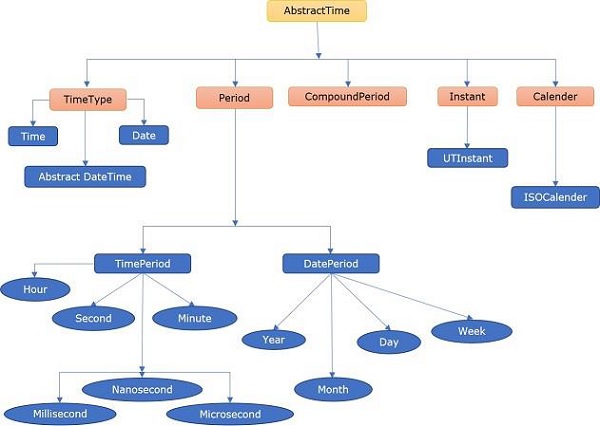
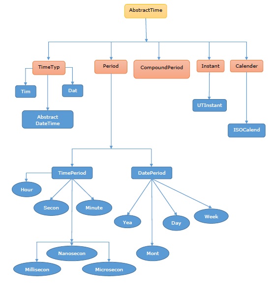
Date, Time, and DateTimes
To work with Dates and Times, Julia has the following three datatypes −
Dates.Time − Accurate to nanosecond, this object represents a precise moment of the day.
Dates.Date − As the name implies, it represents just a date.
Dates.DateTime − Accurate to a millisecond, this object represents combination of a date and a time of day. It actually specifies an exact moment in time.
Example
julia> rightnow = Dates.Time(Dates.now())15:46:39.872julia> My_Birthday = Dates.Date(1984,1,17)1984-01-17julia> armistice_date = Dates.DateTime(1990,11,11,11,11,11)1990-11-11T11:11:11julia> today_date = Dates.today()2020-09-22julia> Dates.now(Dates.UTC)2020-09-22T10:18:32.008julia> Dates.DateTime("20180629 120000", "yyyymmdd HHMMSS")2018-06-29T12:00:00julia> Dates.DateTime("19/07/2007 17:42", "dd/mm/yyyy HH:MM")2007-07-19T17:42:00Queries regrading Date and Time
After having the objects such as date/time or date, we can use the following functions to extract the required information −
julia> Dates.year(My_Birthday)1984julia> Dates.month(My_Birthday)1julia> Dates.minute(now())22julia> Dates.hour(now())19julia> Dates.second(now())19julia> Dates.minute(rightnow)46julia> Dates.hour(rightnow)15julia> Dates.second(rightnow)39julia> Dates.dayofweek(My_Birthday)2julia> Dates.dayname(My_Birthday)"Tuesday"julia> Dates.yearmonthday(My_Birthday)(1984, 1, 17)julia> Dates.dayofweekofmonth(My_Birthday)3
Date Arithmetic
It is also possible to do arithmetic on date/time as well as date objects. The most common one is to find the difference between two such objects as shown in the below example −
Example
julia> today_date - My_Birthday13409 daysjulia> datetimenow - armistice_date943436237800 milliseconds
We can convert these differences in some unit as follows −
julia> Dates.Period(today_date - My_Birthday)13409 daysjulia> Dates.canonicalize(Dates.CompoundPeriod(datetimenow - armistice_date))1559 weeks, 6 days, 9 hours, 37 minutes, 17 seconds, 800 milliseconds
We can also add and subtract periods of time to date and date/time objects as follows −
julia> My_Birthday + Dates.Year(20) + Dates.Month(6)2004-07-17
In the above example, we have added 20 years and 6 months to my birth date.
Range of Dates
Julia provides the facility to create range of dates by making iterable range objects. In the example given below, we will be creating an iterator that yields the first day of every month.
Example
julia> date_range = Dates.Date(2000,1,1):Dates.Month(1):Dates.Date(2020,1,1)Date("2000-01-01"):Month(1):Date("2020-01-01")From the above range object, we can find out which of these fall on weekdays. For this we need to create an anonymous function to filter() which will test the day name against the given day names −
julia> weekdaysfromrange = filter(dy -> Dates.dayname(dy) != "Saturday" && Dates.dayname(dy) != "Sunday" , date_range)171-element Array{Date,1}: 2000-02-01 2000-03-01 2000-05-01 2000-06-01 2000-08-01 2000-09-01 2000-11-01 2000-12-01 2001-01-01 2001-02-01 2001-03-01 2001-05-01 2001-06-01 ⋮ 2018-10-01 2018-11-01 2019-01-01 2019-02-01 2019-03-01 2019-04-01 2019-05-01 2019-07-01 2019-08-01 2019-10-01 2019-11-01 2020-01-01Formatting of Dates
Following table gives the date formatting codes with the help of which we can specify date formats −
| Character | Date/Time element |
|---|---|
| Y | Year digit Ex. yyyy => 1984, yy => 84 |
| m | Month digit Ex. m => 7 or 07 |
| u | Month name Ex. Jun |
| U | Month name Ex. January |
| e | Day of week Ex. Mon |
| E | Day of week Ex. Monday |
| d | Day Ex. 1 or 01 |
| H | Hour digit Ex. HH => 00 |
| M | Minute digit Ex. MM => 00 |
| S | Second digit Ex. S => 00 |
| s | Millisecond digit Ex. .000 |
Example
julia> Dates.Date("Sun, 27 Sep 2020", "e, d u y")2020-09-27julia> Dates.DateTime("Sun, 27 Sep 2020 10:25:10", "e, d u y H:M:S")2020-09-27T10:25:10Rounding Dates and Times
As we know that the functions round(), floor(), and ceil() are usually used to round numbers up or down. These functions can also be used to round dates so that the dates can be adjusted forward or backward in time.
Example
julia> Dates.now()2020-09-27T13:34:03.49julia> Dates.format(round(Dates.DateTime(Dates.now()), Dates.Minute(15)), Dates.RFC1123Format)"Sun, 27 Sep 2020 13:30:00"
The ceil() function will adjust the dates/time forward as given below −
julia> My_Birthday = Dates.Date(1984,1,17)1984-01-17julia> ceil(My_Birthday, Dates.Month)1984-02-01julia> ceil(My_Birthday, Dates.Year)1985-01-01julia> ceil(My_Birthday, Dates.Week)1984-01-23
Recurring Dates
If we want to find all the dates in a range of dates that satisfy some criteria, it is called recurring dates. Let us understand with the help of following example −
First, we need to create a Range of date as we did previously −
julia> date_range = Dates.Date(2000,1,1):Dates.Month(1):Dates.Date(2020,1,1)Date("2000-01-01"):Month(1):Date("2020-01-01")Now we can use filter() function to find Sundays in a month −
julia> filter(d -> Dates.dayname(d) == "Sunday", date_range)35-element Array{Date,1}: 2000-10-01 2001-04-01 2001-07-01 2002-09-01 2002-12-01 2003-06-01 2004-02-01 2004-08-01 2005-05-01 2006-01-01 2006-10-01 2007-04-01 2007-07-01 ⋮ 2013-12-01 2014-06-01 2015-02-01 2015-03-01 2015-11-01 2016-05-01 2017-01-01 2017-10-01 2018-04-01 2018-07-01 2019-09-01 2019-12-01Unix time
Unix time is another type of timekeeping in which the count of the number of seconds that have elapsed since the birth of Unix (beginning of the year 1970). We will never observe the end of Unix time because Julia store the count in a 64-bit integer.
The time() function will return the Unix time value −
julia> using Datesjulia> time()1.60206441103e9
The unix2datetime() function will convert a Unix time value to date/time object −
julia> Dates.unix2datetime(time())2020-09-10T09:54:52.894
Moments in time
DateTimes, in the field instant, are stored in milliseconds. We can obtain this value by using Dates.value function as follows −
julia> moment=Dates.now()2020-09-10T09:56:11.885julia> Dates.value(moment)63737767811885julia> moment.instantDates.UTInstant{Millisecond}(Millisecond(63737767811885))Time and Monitoring
Julia provides us @elapsed macro which will return the time (number of seconds) an expression took to evaluate.
Example
julia> function foo(n) for i in 1:n x = sin(rand()) end endfoo (generic function with 1 method)julia> @elapsed foo(100000000)1.113577001julia> @time foo(100000000)1.134852 seconds
Julia - Files I/O
Reading from files
The functions namely open(), read(), and close() are the standard approach for extracting information from text files.
Opening a text file
If you want to read text from a text file, you need to first obtain the file handle. It can be done with the help of open() function as follows −
foo = open("C://Users//Leekha//Desktop//NLP.txt")It shows that now foo is the Julias connection to the text file namely NLP.txt on the disk.
Closing the file
Once we are done with the file, we should have to close the connection as follows −
Close(foo)
In Julia, it is recommended to wrap any file-processing functions inside a do block as follows −
open("NLP.txt") do file # here you can work with the open fileendThe advantage of wrapping file-processing functions inside do block is that the open file will be automatically closed when this block finishes.
An example to keep some of the information like total time to read the file and total lines in the files −
julia> totaltime, totallines = open("C://Users//Leekha//Desktop//NLP.txt") do foo linecounter = 0 timetaken = @elapsed for l in eachline(foo) linecounter += 1 end (timetaken, linecounter) end(0.0001184, 87)Reading a file all at once
With read() function, we can read the whole content of an open file at once, for example −
ABC = read(foo, String)
Similarly, the below will store the contents of the file in ABC −
julia> ABC = open("C://Users//Leekha//Desktop//NLP.txt") do file read(file, String) endWe can also read in the whole file as an array. Use readlines() as follows −
julia> foo = open("C://Users//Leekha//Desktop//NLP.txt")IOStream(<file C://Users//Leekha//Desktop//NLP.txt>)julia> lines = readlines(foo)87-element Array{String,1}: "Natural Language Processing: Semantic Analysis " "" "Introduction to semantic analysis:""The purpose of semantic analysis is to draw exact meaning, or you can say dictionary meaning from the text. Semantic analyzer checks the text for meaningfulness. "Reading line by line
We can also process a file line by line. For this task, Julia provides a function named eachline() which basically turns a source into an iterator.
julia> open("C://USers/Leekha//Desktop//NLP.txt") do file for ln in eachline(file) println("$(length(ln)), $(ln)") end end47, Natural Language Processing: Semantic Analysis0,34, Introduction to semantic analysis:If you want to keep a track of which line you are on while reading the file, use the below given approach −
julia> open("C://Users//Leekha//Desktop//NLP.txt") do f line = 1 while !eof(f) x = readline(f) println("$line $x") line += 1 end end1 Natural Language Processing: Semantic Analysis23 Introduction to semantic analysis:4 The purpose of semantic analysis is to draw exact meaning, or you can say dictionary meaning from the text. Semantic analyzer checks the text for meaningfulness.5 We know that lexical analysis also deals with the meaning of the words then how semantic analysis is different from lexical analysis? The answer is that Lexical analysis is based on smaller token but on the other side semantic analysis focuses on larger chunks. That is why semantic analysis can be divided into the following two parts:6 Studying the meaning of individual word: It is the first part of the semantic analysis in which the study of the meaning of individual words is performed. This part is called lexical semantics.7 Studying the combination of individual words: In this second part, the individual words will be combined to provide meaning in sentences.8 The most important task of semantic analysis is to get the proper meaning of the sentence. For example, analyze the sentence Ram is great. In this sentence, the speaker is talking either about Lord Ram or about a person whose name is Ram. That is why the job, to get the proper meaning of the sentence, of semantic analyzer is important.9 Elements of semantic analysis:10 Following are the elements of semantic analysis:..Path and File Names
The table below shows functions that are useful for working with filenames −
| Sl.No | Functions & Working |
|---|---|
| 1 | cd(path) This function changes the current directory. |
| 2 | pwd() This function gets the current working directory. |
| 3 | readdir(path) This function returns a list of the contents of a named directory, or the current directory. |
| 4 | abspath(path) This function adds the current directory's path to a filename to make an absolute pathname. |
| 5 | joinpath(str, str, ...) This function assembles a pathname from pieces. |
| 6 | isdir(path) This function tells you whether the path is a directory. |
| 7 | splitdir(path) This function splits a path into a tuple of the directory name and file name. |
| 8 | splitdrive(path) This function, on Windows, split a path into the drive letter part and the path part. And, On Unix systems, the first component is always the empty string. |
| 9 | splitext(path) This function, if the last component of a path contains a dot, split the path into everything before the dot and everything including and after the dot. Otherwise, return a tuple of the argument unmodified and the empty string. |
| 10 | expanduser(path) This function replaces a tilde character at the start of a path with the current user's home directory. |
| 11 | normpath(path) This function normalizes a path, removing "." and ".." entries. |
| 12 | realpath(path) This function canonicalizes a path by expanding symbolic links and removing "." and ".." entries. |
| 13 | homedir() This function gives the current user's home directory. |
| 14 | dirname(path) This function gets the directory part of a path. |
| 15 | basename(path) This function gets the file name part of a path. |
Information about file
We can use stat(pathname) to get the information about a specific file.
Example
julia> for n in fieldnames(typeof(stat("C://Users//Leekha//Desktop//NLP.txt"))) println(n, ": ", getfield(stat("C://Users//Leekha//Desktop//NLP.txt"),n)) enddevice: 3262175189inode: 17276mode: 33206nlink: 1uid: 0gid: 0rdev: 0size: 6293blksize: 4096blocks: 16mtime: 1.6017034024103658e9ctime: 1.6017034024103658e9Interacting with the file system
If you want to convert filenames to pathnames, you can use abspath() function. We can map this over a list of files in a directory as follows −
julia> map(abspath, readdir())204-element Array{String,1}: "C:\\Users\\Leekha\\.anaconda" "C:\\Users\\Leekha\\.conda" "C:\\Users\\Leekha\\.condarc" "C:\\Users\\Leekha\\.config" "C:\\Users\\Leekha\\.idlerc" "C:\\Users\\Leekha\\.ipynb_checkpoints" "C:\\Users\\Leekha\\.ipython" "C:\\Users\\Leekha\\.julia" "C:\\Users\\Leekha\\.jupyter" "C:\\Users\\Leekha\\.keras" "C:\\Users\\Leekha\\.kindle"Writing to files
A function writedlm(), a function in the DelimitedFiles package can be used to write the contents of an object to a text file.
Example
julia> test_numbers = rand(10,10)1010 Array{Float64,2}: 0.457071 0.41895 0.63602 0.812757 0.727214 0.156181 0.023817 0.286904 0.488069 0.232787 0.623791 0.946815 0.757186 0.822932 0.791591 0.67814 0.903542 0.664997 0.702893 0.924639 0.334988 0.511964 0.738595 0.631272 0.33401 0.634704 0.175641 0.0679822 0.350901 0.0773231 0.838656 0.140257 0.404624 0.346231 0.642377 0.404291 0.888538 0.356232 0.924593 0.791257 0.438514 0.70627 0.642209 0.196252 0.689652 0.929208 0.19364 0.19769 0.868283 0.258201 0.599995 0.349388 0.22805 0.0180824 0.0226505 0.0838017 0.363375 0.725694 0.224026 0.440138 0.526417 0.788251 0.866562 0.946811 0.834365 0.173869 0.279936 0.80839 0.325284 0.0737317 0.0805326 0.507168 0.388336 0.186871 0.612322 0.662037 0.331884 0.329227 0.355914 0.113426 0.527173 0.0799835 0.543556 0.332768 0.105341 0.409124 0.61811 0.623762 0.944456 0.0490737 0.281633 0.934487 0.257375 0.409263 0.206078 0.720507 0.867653 0.571467 0.705971 0.11014 julia> writedlm("C://Users//Leekha//Desktop//testfile.txt", test_numbers)Julia Programming - Metaprogramming
Metaprogramming may be defined as the programming in which we write Julia code to process and modify Julia code. With the help of Julia metaprogramming tools, one can write Julia programming code that modifies other parts of the source code file. These tools can even control when the modified code runs.
Following are the execution stages of raw source code −
Stage 1 − Raw Julia code is parsed
In this stage the raw Julia code is converted into a form suitable for evaluation. The output of this stage is AST i.e. Abstract Syntax Tree. AST is a structure which contains all the code in an easy to manipulate format.
Stage 2 − Parsed Julia code is executed
In this stage, the evaluated Julia code is executed. When we type code in REPL and press Return the two stages happens but they happen so quickly that we dont even notice. But with metaprogramming tools we can access the Julia code between two stages, i.e. after code parsed but before its evaluation.
Quoted expressions
As we discussed, with metaprogramming we can access the Julia code between two stages. For this, Julia has : colon prefix operator. With the help of colon operator, Julia store an unevaluated but parsed expression.
Example
julia> ABC = 100 100 julia> :ABC:ABC
Here, − ABC is quoted or unevaluated symbol for Julia i.e. ABC is an unevaluated symbol rather than having the value 100.
We can quote the whole expressions as below −
julia> :(100-50):(100 - 50)
Alternatively, we can also use quoteend keywords to enclose and quote an expression as follows −
julia> quote 100 - 50 endquote #= REPL[43]:2 =# 100 - 50endCheck this also:julia> expression = quote for x = 1:5 println(x) end endquote #= REPL[46]:2 =# for x = 1:5 #= REPL[46]:3 =# println(x) endendjulia> typeof(expression)Expr
It shows that expression object is parsed, primed and ready to use.
Evaluated expressions
Once you parsed the expression, there is a way to evaluate the expression also. We can use the function eval() for this purpose as follows −
julia> eval(:ABC)100julia> eval(:(100-50))50julia> eval(expression)12345
In the example, we have evaluated the expressions parsed in above section.
The Abstract Syntax Tree (AST)
As discussed above, Abstract Syntax Tree (AST) is a structure which contains all the code in an easy to manipulate format. It is the output of stage1. It allows us to easily process and modify the Julia code. We can visualize the hierarchical nature of an expression with the help of dump() function.
Example
julia> dump(:(1 * cos(pi/2)))Expr head: Symbol call args: Array{Any}((3,)) 1: Symbol * 2: Int64 1 3: Expr head: Symbol call args: Array{Any}((2,)) 1: Symbol cos 2: Expr head: Symbol call args: Array{Any}((3,)) 1: Symbol / 2: Symbol pi 3: Int64 2Expression interpolation
Any Julia code which has string or expression is usually unevaluated but with the help of dollar ($) sign (string interpolation operator), we can evaluate some of the code. The Julia code will be evaluated and inserts the resulting value into the string when the string interpolation operator is used inside a string.
Example
julia> "the cosine of 1 is $(cos(1))""the cosine of 1 is 0.5403023058681398"
Similarly, we can use this string interpolation operator to include the results of executing Julia code interpolated into unevaluated expression −
julia> quote ABC = $(cos(1) + tan(1)); endquote #= REPL[54]:1 =# ABC = 2.097710030523042end
Macros
We are now aware of creating and handling unevaluated expressions. In this section, we will understand how we can modify them. Julia provides macro that accepts an unevaluated expression as input and generates a new output expression.
If we talk about its working, Julia first parses and evaluates the macro, and then the processed code produced by macro will be evaluated like an ordinary expression.
The syntax of defining a macro is very similar to that of a function. Following is the definition of macro that will print out the contents of the things we pass to it −
julia> macro x(n) if typeof(n) == Expr println(n.args) end return n end@x (macro with 1 method)
We can run the macros by preceding the name of the macro with the @ prefix −
julia> @x 500500julia> @x "Tutorialspoint.com""Tutorialspoint.com"eval() and @eval
Julia has eval() function and a macro called @eval. Let us see example to know their differences −
julia> ABC = :(100 + 50):(100 + 50)julia> eval(ABC)150
The above output shows that the eval() function expands the expression and evaluates it.
julia> @eval ABC:(100 + 50)julia> @eval $(ABC)150
It can also be treated as follows −
julia> @eval $(ABC) == eval(ABC)true
Expanding Macros
The macroexpand() function returns the expanded format (used by the Julia compiler before it is finally executed) of the specified macro.
Example
julia> macroexpand(Main, quote @p 1 + 4 - 6 * 7 / 8 % 9 end)Any[:-, :(1 + 4), :(((6 * 7) / 8) % 9)]quote #= REPL[69]:1 =# (1 + 4) - ((6 * 7) / 8) % 9end
Julia Programming - Plotting
Julia has various packages for plotting and before starting making plots, we need to first download and install some of them as follows −
(@v1.5) pkg> add Plots PyPlot GR UnicodePlots
The package Plots is a high-level plotting package, also referred to as back-ends interfaces with other plotting packages. To start using the Plots package, type the following command −
julia> using Plots[ Info: Precompiling Plots [91a5bcdd-55d7-5caf-9e0b-520d859cae80]
Plotting a function
For plotting a function, we need to switch back to PyPlot back-end as follows −
julia> pyplot()Plots.PyPlotBackend()
Here we will be plotting the equation of Time graph which can be modeled by the following function −
julia> eq(d) = -7.65 * sind(d) + 9.87 * sind(2d + 206);julia> plot(eq, 1:365)sys:1: MatplotlibDeprecationWarning: Passing the fontdict parameter of _set_ticklabels() positionally is deprecated since Matplotlib 3.3; the parameter will become keyword-only two minor releases later.sys:1: UserWarning: FixedFormatter should only be used together with FixedLocator
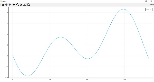
Packages
Everyone wants a package that helps them to draw quick plots by text rather than graphics.
UnicodePlots
Julia provides one such package called UnicodePlots which can produce the following −
scatter plots
line plots
bar plots
staircase plots
histograms
sparsity patterns
density plots
We can add it to our Julia installation by the following command −
(@v1.5) pkg> add UnicodePlots
Once added, we can use this to plot a graph as follows:
julia> using UnicodePlots
Example
Following Julia example generates a line chart using UnicodePlots.
julia> FirstLinePlot = lineplot([1, 2, 3, 7], [1, 2, -5, 7], title="First Line Plot", border=:dotted) First Line Plot
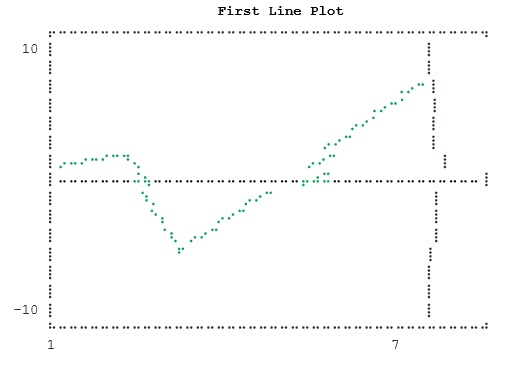
Example
Following Julia example generates a density chart using UnicodePlots.
Julia> using UnicodePlotsJulia> FirstDensityPlot = densityplot(collect(1:100), randn(100), border=:dotted)
VegaLite
This Julia package is a visualization grammar which allows us to create visualization in a web browser window. With this package, we can −
describe data visualization in a JSON format
generate interactive views using HTML5 Canvas or SVG
It can produce the following −
Area plots
Bar plots/Histograms
Line plots
Scatter plots
Pie/Donut charts
Waterfall charts
Worldclouds
We can add it to our Julia installation by following command −
(@v1.5) pkg> add VegaLite
Once added we can use this to plot a graph as follows −
julia> using VegaLite
Example
Following Julia example generates a Pie chart using VegaLite.
julia> X = ["Monday", "Tuesday", "Wednesday", "Thrusday", "Friday","Saturday","Sunday"];julia> Y = [11, 11, 15, 13, 12, 13, 10]7-element Array{Int64,1}: 11 11 15 13 12 13 10 julia> P = pie(X,Y)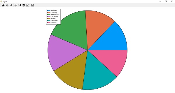
Julia Programming - Data Frames
DataFrame may be defined as a table or spreadsheet which we can be used to sort as well as explore a set of related data values. In other words, we can call it a smarter array for holding tabular data. Before we use it, we need to download and install DataFrame and CSV packages as follows −
(@v1.5) pkg> add DataFrames(@v1.5) pkg> add CSV
To start using the DataFrames package, type the following command −
julia> using DataFrames
Loading data into DataFrames
There are several ways to create new DataFrames (which we will discuss later in this section) but one of the quickest ways to load data into DataFrames is to load the Anscombe dataset. For better understanding, let us see the example below −
anscombe = DataFrame( [10 10 10 8 8.04 9.14 7.46 6.58; 8 8 8 8 6.95 8.14 6.77 5.76; 13 13 13 8 7.58 8.74 12.74 7.71; 9 9 9 8 8.81 8.77 7.11 8.84; 11 11 11 8 8.33 9.26 7.81 8.47; 14 14 14 8 9.96 8.1 8.84 7.04; 6 6 6 8 7.24 6.13 6.08 5.25; 4 4 4 19 4.26 3.1 5.39 12.5; 12 12 12 8 10.84 9.13 8.15 5.56; 7 7 7 8 4.82 7.26 6.42 7.91; 5 5 5 8 5.68 4.74 5.73 6.89]);
julia> rename!(anscombe, [Symbol.(:N, 1:4); Symbol.(:M, 1:4)])118 DataFrame Row N1 N2 N3 N4 M1 M2 M3 M4 Float64 Float64 Float64 Float64 Float64 Float64 Float64 Float64 1 10.0 10.0 10.0 8.0 8.04 9.14 7.46 6.58 2 8.0 8.0 8.0 8.0 6.95 8.14 6.77 5.76 3 13.0 13.0 13.0 8.0 7.58 8.74 12.74 7.71 4 9.0 9.0 9.0 8.0 8.81 8.77 7.11 8.84 5 11.0 11.0 11.0 8.0 8.33 9.26 7.81 8.47 6 14.0 14.0 14.0 8.0 9.96 8.1 8.84 7.04 7 6.0 6.0 6.0 8.0 7.24 6.13 6.08 5.25 8 4.0 4.0 4.0 19.0 4.26 3.1 5.39 12.5 9 12.0 12.0 12.0 8.0 10.84 9.13 8.15 5.56 10 7.0 7.0 7.0 8.0 4.82 7.26 6.42 7.91 11 5.0 5.0 5.0 8.0 5.68 4.74 5.73 6.89
We assigned the DataFrame to a variable named Anscombe, convert them to an array and then rename columns.
Collected Datasets
We can also use another dataset package named RDatasets package. It contains several other famous datasets including Anscombes. Before we start using it, we need to first download and install it as follows −
(@v1.5) pkg> add RDatasets
To start using this package, type the following command −
julia> using DataFramesjulia> anscombe = dataset("datasets","anscombe")118 DataFrame Row X1 X2 X3 X4 Y1 Y2 Y3 Y4 Int64 Int64 Int64 Int64 Float64 Float64 Float64 Float64 1 10 10 10 8 8.04 9.14 7.46 6.58 2 8 8 8 8 6.95 8.14 6.77 5.76 3 13 13 13 8 7.58 8.74 12.74 7.71 4 9 9 9 8 8.81 8.77 7.11 8.84 5 11 11 11 8 8.33 9.26 7.81 8.47 6 14 14 14 8 9.96 8.1 8.84 7.04 7 6 6 6 8 7.24 6.13 6.08 5.25 8 4 4 4 19 4.26 3.1 5.39 12.5 9 12 12 12 8 10.84 9.13 8.15 5.56 10 7 7 7 8 4.82 7.26 6.42 7.91 11 5 5 5 8 5.68 4.74 5.73 6.89 Empty DataFrames
We can also create DataFrames by simply providing the information about rows, columns as we give in an array.
Example
julia> empty_df = DataFrame(X = 1:10, Y = 21:30)102 DataFrame Row X Y Int64 Int64 1 1 21 2 2 22 3 3 23 4 4 24 5 5 25 6 6 26 7 7 27 8 8 28 9 9 29 10 10 30
To create completely empty DataFrame, we only need to supply the Column Names and define their types as follows −
julia> Complete_empty_df = DataFrame(Name=String[], W=Float64[], H=Float64[], M=Float64[], V=Float64[])05 DataFrame
julia> Complete_empty_df = vcat(Complete_empty_df, DataFrame(Name="EmptyTestDataFrame", W=5.0, H=5.0, M=3.0, V=5.0))15 DataFrame Row Name W H M V String Float64 Float64 Float64 Float64 1 EmptyTestDataFrame 5.0 5.0 3.0 5.0
julia> Complete_empty_df = vcat(Complete_empty_df, DataFrame(Name="EmptyTestDataFrame2", W=6.0, H=6.0, M=5.0, V=7.0))25 DataFrame Row Name W H M V String Float64 Float64 Float64 Float64 1 EmptyTestDataFrame 5.0 5.0 3.0 5.0 2 EmptyTestDataFrame2 6.0 6.0 5.0 7.0
Plotting Anscombes Quarter
Now the Anscombe dataset has been loaded, we can do some statistics with it also. The inbuilt function named describe() enables us to calculate the statistics properties of the columns of a dataset. You can supply the symbols, given below, for the properties −
mean
std
min
q25
median
q75
max
eltype
nunique
first
last
nmissing
Example
julia> describe(anscombe, :mean, :std, :min, :median, :q25)86 DataFrame Row variable mean std min median q25 Symbol Float64 Float64 Real Float64 Float64 1 X1 9.0 3.31662 4 9.0 6.5 2 X2 9.0 3.31662 4 9.0 6.5 3 X3 9.0 3.31662 4 9.0 6.5 4 X4 9.0 3.31662 8 8.0 8.0 5 Y1 7.50091 2.03157 4.26 7.58 6.315 6 Y2 7.50091 2.03166 3.1 8.14 6.695 7 Y3 7.5 2.03042 5.39 7.11 6.25 8 Y4 7.50091 2.03058 5.25 7.04 6.17
We can also do a comparison between XY datasets as follows −
julia> [describe(anscombe[:, xy], :mean, :std, :median, :q25) for xy in [[:X1, :Y1], [:X2, :Y2], [:X3, :Y3], [:X4, :Y4]]]4-element Array{DataFrame,1}:25 DataFrame Row variable mean std median q25 Symbol Float64 Float64 Float64 Float64 1 X1 9.0 3.31662 9.0 6.5 2 Y1 7.50091 2.03157 7.58 6.315 25 DataFrame Row variable mean std median q25 Symbol Float64 Float64 Float64 Float64 1 X2 9.0 3.31662 9.0 6.5 2 Y2 7.50091 2.03166 8.14 6.695 25 DataFrame Row variable mean std median q25 Symbol Float64 Float64 Float64 Float64 1 X3 9.0 3.31662 9.0 6.5 2 Y3 7.5 2.03042 7.11 6.25 25 DataFrame Row variable mean std median q25 Symbol Float64 Float64 Float64 Float64 1 X4 9.0 3.31662 8.0 8.0 2 Y4 7.50091 2.03058 7.04 6.17 Let us reveal the true purpose of Anscombe, i.e., plot the four sets of its quartet as follows −
julia> using StatsPlots[ Info: Precompiling StatsPlots [f3b207a7-027a-5e70-b257-86293d7955fd]julia> @df anscombe scatter([:X1 :X2 :X3 :X4], [:Y1 :Y2 :Y3 :Y4], smooth=true, line = :red, linewidth = 2, title= ["X$i vs Y$i" for i in (1:4)'], legend = false, layout = 4, xlimits = (2, 20), ylimits = (2, 14))
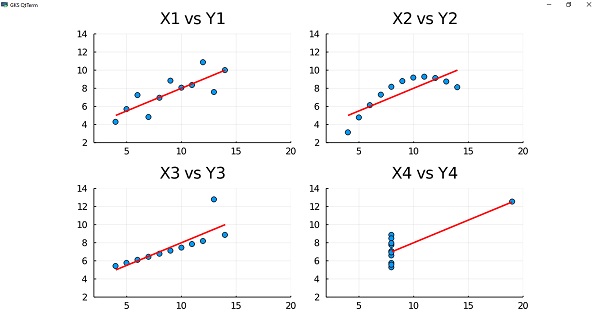
Regression and Models
In this section, we will be working with Linear Regression line for the dataset. For this we need to use Generalized Linear Model (GLM) package which you need to first add as follows −
(@v1.5) pkg> add GLM
Now let us create a liner regression model by specifying a formula using the @formula macro and supplying columns names as well as name of the DataFrame. An example for the same is given below −
julia> linearregressionmodel = fit(LinearModel, @formula(Y1 ~ X1), anscombe)StatsModels.TableRegressionModel{LinearModel{GLM.LmResp{Array{Float64,1}},GLM.DensePredChol{Float64,LinearAlgebra.Cholesky{Float64,Array{Float64,2}}}},Array{Float64,2}}Y1 ~ 1 + X1Coefficients: Coef. Std. Error t Pr(>|t|) Lower 95% Upper 95%(Intercept) 3.00009 1.12475 2.67 0.0257 0.455737 5.54444 X1 0.500091 0.117906 4.24 0.0022 0.23337 0.766812Let us check the summary and the coefficient of the above created linear regression model −
julia> summary(linearregressionmodel)"StatsModels.TableRegressionModel{LinearModel{GLM.LmResp{Array{Float64,1}},GLM.DensePredChol{Float64,LinearAlgebra.Cholesky{Float64,Array{Float64,2}}}},Array{Float64,2}}"julia> coef(linearregressionmodel)2-element Array{Float64,1}: 3.0000909090909054 0.5000909090909096Now let us produce a function for the regression line. The form of the function is y = ax +c.
julia> f(x) = coef(linearmodel)[2] * x + coef(linearmodel)[1]f (generic function with 1 method)
Once we have the function that describes the regression line, we can draw a plot as follows −
julia> p1 = plot(anscombe[:X1], anscombe[:Y1], smooth=true, seriestype=:scatter, title = "X1 vs Y1", linewidth=8, linealpha=0.5, label="data") julia> plot!(f, 2, 20, label="correlation")
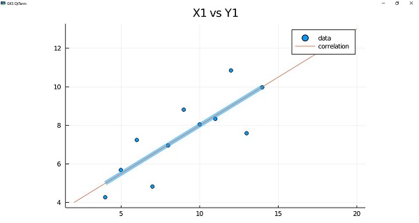
Working with DataFrames
As we know that nothing is perfect. This is also true in case of datasets because not all the datasets are consistent and tidy. To show how we can work with different items of DataFrame, let us create a test DataFrame −
julia> testdf = DataFrame( Number = [3, 5, 7, 8, 20 ], Name = ["Lithium", "Boron", "Nitrogen", "Oxygen", "Calcium" ], AtomicWeight = [6.941, 10.811, 14.0067, 15.9994, 40.078 ], Symbol = ["Li", "B", "N", "O", "Ca" ], Discovered = [1817, 1808, 1772, 1774, missing ])55 DataFrame Row Number Name AtomicWeight Symbol Discovered Int64 String Float64 String Int64? 1 3 Lithium 6.941 Li 1817 2 5 Boron 10.811 B 1808 3 7 Nitrogen 14.0067 N 1772 4 8 Oxygen 15.9994 O 1774 5 20 Calcium 40.078 Ca missing
Handling missing values
There can be some missing values in datasets. It can be checked with the help of describe() function as follows −
julia> describe(testdf)58 DataFrame Row variable mean min median max nunique nmissing eltype Symbol Union Any Union Any Union Union Type 1 Number 8.6 3 7.0 20 Int64 2 Name Boron Oxygen 5 String 3 AtomicWeight 17.5672 6.941 14.0067 40.078 Float64 4 Symbol B O 5 String 5 Discovered 1792.75 1772 1791.0 1817 1 Union{Missing, Int64} Julia provides a special datatype called Missing to address such issue. This datatype indicates that there is not a usable value at this location. That is why the DataFrames packages allow us to get most of our datasets and make sure that the calculations are not tampered due to missing values.
Looking for missing values
We can check with ismissing() function that whether the DataFrame has any missing value or not.
Example
julia> for row in 1:nrows for col in 1:ncols if ismissing(testdf [row,col]) println("$(names(testdf)[col]) value for $(testdf[row,:Name]) is missing!") end end endDiscovered value for Calcium is missing!
Repairing DataFrames
We can use the following code to change values that are not acceptable like n/a, 0, missing. The below code will look in every cell for above mentioned non-acceptable values.
Example
julia> for row in 1:size(testdf, 1) # or nrow(testdf) for col in 1:size(testdf, 2) # or ncol(testdf) println("processing row $row column $col ") temp = testdf [row,col] if ismissing(temp) println("skipping missing") elseif temp == "n/a" || temp == "0" || temp == 0 testdf [row, col] = missing println("changed row $row column $col ") end end endprocessing row 1 column 1processing row 1 column 2processing row 1 column 3processing row 1 column 4processing row 1 column 5processing row 2 column 1processing row 2 column 2processing row 2 column 3processing row 2 column 4processing row 2 column 5processing row 3 column 1processing row 3 column 2processing row 3 column 3processing row 3 column 4processing row 3 column 5processing row 4 column 1processing row 4 column 2processing row 4 column 3processing row 4 column 4processing row 4 column 5processing row 5 column 1processing row 5 column 2processing row 5 column 3processing row 5 column 4processing row 5 column 5skipping missingWorking with missing values
Julia provides support for representing missing values in the statistical sense, that is for situations where no value is available for a variable in an observation, but a valid value theoretically exists.
completecases()
The completecases() function is used to find the maximum value of the column that contains the missing value.
Example
julia> maximum(testdf[completecases(testdf), :].Discovered)1817
dropmissing()
The dropmissing() function is used to get the copy of DataFrames without having the missing values.
Example
julia> dropmissing(testdf)45 DataFrame Row Number Name AtomicWeight Symbol Discovered Int64 String Float64 String Int64 1 3 Lithium 6.941 Li 1817 2 5 Boron 10.811 B 1808 3 7 Nitrogen 14.0067 N 1772 4 8 Oxygen 15.9994 O 1774
Modifying DataFrames
The DataFrames package of Julia provides various methods using which you can add, remove, rename columns, and add/delete rows.
Adding Columns
We can use hcat() function to add a column of integers to the DataFrame. It can be used as follows −
julia> hcat(testdf, axes(testdf, 1))56 DataFrame Row Number Name AtomicWeight Symbol Discovered x1 Int64 String Float64 String Int64? Int64 1 3 Lithium 6.941 Li 1817 1 2 5 Boron 10.811 B 1808 2 3 7 Nitrogen 14.0067 N 1772 3 4 8 Oxygen 15.9994 O 1774 4 5 20 Calcium 40.078 Ca missing 5
But as you can notice that we havent changed the DataFrame or assigned any new DataFrame to a symbol. We can add another column as follows −
julia> testdf [!, :MP] = [180.7, 2300, -209.86, -222.65, 839]5-element Array{Float64,1}: 180.7 2300.0 -209.86 -222.65 839.0julia> testdf56 DataFrame Row Number Name AtomicWeight Symbol Discovered MP Int64 String Float64 String Int64? Float64 1 3 Lithium 6.941 Li 1817 180.7 2 5 Boron 10.811 B 1808 2300.0 3 7 Nitrogen 14.0067 N 1772 -209.86 4 8 Oxygen 15.9994 O 1774 -222.65 5 20 Calcium 40.078 Ca missing 839.0 We have added a column having melting points of all the elements to our test DataFrame.
Removing Columns
We can use select!() function to remove a column from the DataFrame. It will create a new DataFrame that contains the selected columns, hence to remove a particular column, we need to use select!() with Not. It is shown in the given example −
julia> select!(testdf, Not(:MP))55 DataFrame Row Number Name AtomicWeight Symbol Discovered Int64 String Float64 String Int64? 1 3 Lithium 6.941 Li 1817 2 5 Boron 10.811 B 1808 3 7 Nitrogen 14.0067 N 1772 4 8 Oxygen 15.9994 O 1774 5 20 Calcium 40.078 Ca missing
We have removed the column MP from our Data Frame.
Renaming Columns
We can use rename!() function to rename a column in the DataFrame. We will be renaming the AtomicWeight column to AW as follows −
julia> rename!(testdf, :AtomicWeight => :AW)55 DataFrame Row Number Name AW Symbol Discovered Int64 String Float64 String Int64? 1 3 Lithium 6.941 Li 1817 2 5 Boron 10.811 B 1808 3 7 Nitrogen 14.0067 N 1772 4 8 Oxygen 15.9994 O 1774 5 20 Calcium 40.078 Ca missing
Adding rows
We can use push!() function with suitable data to add rows in the DataFrame. In the below given example we will be adding a row having element Cooper −
Example
julia> push!(testdf, [29, "Copper", 63.546, "Cu", missing])65 DataFrame Row Number Name AW Symbol Discovered Int64 String Float64 String Int64? 1 3 Lithium 6.941 Li 1817 2 5 Boron 10.811 B 1808 3 7 Nitrogen 14.0067 N 1772 4 8 Oxygen 15.9994 O 1774 5 20 Calcium 40.078 Ca missing 6 29 Copper 63.546 Cu missing
Deleting rows
We can use deleterows!() function with suitable data to delete rows from the DataFrame. In the below given example we will be deleting three rows (4th, 5th,and 6th) from our test data frame −
Example
julia> deleterows!(testdf, 4:6)35 DataFrame Row Number Name AW Symbol Discovered Int64 String Float64 String Int64? 1 3 Lithium 6.941 Li 1817 2 5 Boron 10.811 B 1808 3 7 Nitrogen 14.0067 N 1772
Finding values in DataFrame
To find the values in DataFrame, we need to use an elementwise operator examining all the rows. This operator will return an array of Boolean values to indicate whether cells meet the criteria or not.
Example
julia> testdf[:, :AW] .< 103-element BitArray{1}:100julia> testdf[testdf[:, :AW] .< 10, :]15 DataFrame Row Number Name AW Symbol Discovered Int64 String Float64 String Int64? 1 3 Lithium 6.941 Li 1817 Sorting
To sort the values in DataFrame, we can use sort!() function. We need to give the columns on which we want to sort.
Example
julia> sort!(testdf, [order(:AW)])35 DataFrame Row Number Name AW Symbol Discovered Int64 String Float64 String Int64? 1 3 Lithium 6.941 Li 1817 2 5 Boron 10.811 B 1808 3 7 Nitrogen 14.0067 N 1772
The DataFrame is sorted based on the values of column AW.
Julia Programming - Working with Datasets
In this chapter, we shall discuss in detail about datasets.
CSV files
As we know that CSV (Comma Separated Value) file is a plain text file which uses commas to separate fields and values of those fields. The extension of these files is .CSV. We have various methods provided by Julia programming language to perform operations on CSV files.
Import a .CSV file in Julia
To import a .CSV file, we need to install CSV package. Use the following command to do so −
using pkgpkg.add("CSV")Reading data
To read data from a CSV file in Julia we need to use read() method from CSV package as follows −
julia> using CSVjulia> CSV.read("C://Users//Leekha//Desktop//Iris.csv")1506 DataFrame Row Id SepalLengthCm SepalWidthCm PetalLengthCm PetalWidthCm Species Int64 Float64 Float64 Float64 Float64 String ------- 1 1 5.1 3.5 1.4 0.2 Iris-setosa 2 2 4.9 3.0 1.4 0.2 Iris-setosa 3 3 4.7 3.2 1.3 0.2 Iris-setosa 4 4 4.6 3.1 1.5 0.2 Iris-setosa 5 5 5.0 3.6 1.4 0.2 Iris-setosa 6 6 5.4 3.9 1.7 0.4 Iris-setosa 7 7 4.6 3.4 1.4 0.3 Iris-setosa 8 8 5.0 3.4 1.5 0.2 Iris-setosa 9 9 4.4 2.9 1.4 0.2 Iris-setosa 10 10 4.9 3.1 1.5 0.1 Iris-setosa ⋮ 140 140 6.9 3.1 5.4 2.1 Iris-virginica 141 141 6.7 3.1 5.6 2.4 Iris-virginica 142 142 6.9 3.1 5.1 2.3 Iris-virginica 143 143 5.8 2.7 5.1 1.9 Iris-virginica 144 144 6.8 3.2 5.9 2.3 Iris-virginica 145 145 6.7 3.3 5.7 2.5 Iris-virginica 146 146 6.7 3.0 5.2 2.3 Iris-virginica 147 147 6.3 2.5 5.0 1.9 Iris-virginica 148 148 6.5 3.0 5.2 2.0 Iris-virginica 149 149 6.2 3.4 5.4 2.3 Iris-virginica 150 150 5.9 3.0 5.1 1.8 Iris-virginica Creating new CSV file
To create new CSV file, we need to use touch()command from CSV package. We also need to use DataFrames package to write the newly created content to new CSV file −
julia> using DataFramesjulia> using CSVjulia> touch("1234.csv")"1234.csv"julia> new = open("1234.csv", "w")IOStream(<file 1234.csv>)julia> new_data = DataFrame(Name = ["Gaurav", "Rahul", "Aarav", "Raman", "Ravinder"], RollNo = [1, 2, 3, 4, 5], Marks = [54, 67, 90, 23, 95]) 53 DataFrame Row Name RollNo Marks String Int64 Int64 1 Gaurav 1 54 2 Rahul 2 67 3 Aarav 3 90 4 Raman 4 23 5 Ravinder 5 95 julia> CSV.write("1234.csv", new_data)"1234.csv"julia> CSV.read("1234.csv")53 DataFrame Row Name RollNo Marks String Int64 Int64 1 Gaurav 1 54 2 Rahul 2 67 3 Aarav 3 90 4 Raman 4 23 5 Ravinder 5 95 HDF5
The full form of HDF5 is Hierarchical Data Format v5. Following are some of its properties −
A group is similar to a directory, a dataset is like a file.
To associate metadata with a particular group, it uses attributes.
It uses ASCII names for different objects.
Language wrappers are often known as low level or high level.
Opening HDF5 files
HDF5 files can be opened with h5open command as follows −
fid = h5open(filename, mode)
Following table describes the mode −
| Sl.No | Mode & Meaning |
|---|---|
| 1 | "r" read-only |
| 2 | "r+" read-write − It will preserve any existing contents. |
| 3 | "cw" read-write − It will create file if not existing. It will also preserve existing contents. |
| 4 | "w" read-write − It will destroy any existing contents. |
The above command will produce an object of type HDF5File and a subtype of the abstract type DataFile.
Closing HDF5 files
Once finished with a file, we should close it as follows −
close(fid)
It will also close all the objects in the file.
Opening HDF5 objects
Suppose if we have a file object named fid and it has a group called object1, it can be opened as follows −
Obj1 = fid[object1]
Closing HDF5 objects
close(obj1)
Reading data
A group g containing a dataset with path dtset and we have opened dataset as dset1 = g[dtset]. We can read the information in following ways −
ABC = read(dset1)ABC = read(g, "dtset")Asub = dset1[2:3, 1:3]
Writing data
We can create the dataset as follows −
g["dset1"] = rand(3,5)write(g, "dset1", rand(3,5))
XML files
Here we will be discussing about LightXML.jl package which is a light-weight Julia wrapper for libxml2. It provides the following functionalities −
Parsing an XML file
Accessing XML tree structure
Creating an XML tree
Exporting an XML tree to a string
Example
Suppose we have an xml file named new.xml as follows −
<Hello> <to>Gaurav</to> <from>Rahul</from> <heading>Reminder to meet</heading> <body>Friend, Don't forget to meet this weekend!</body></Hello>
Now, we can parse this file by using LightXML as follows −
julia> using LightXML#below code will parse this xml filejulia> xdoc = parse_file("C://Users//Leekha//Desktop//new.xml")<?xml version="1.0" encoding="utf-8"?><Hello><to>Gaurav</to><from>Rahul</from><heading>Reminder to meet</heading><body>Friend, Don't forget to meet this weekend!</body></Hello>Following example explains how to get the root element −
julia> xroot = root(xdoc);julia> println(name(xroot))Hello#Traversing all the child nodes and also print element namesjulia> for c in child_nodes(xroot) # c is an instance of XMLNode println(nodetype(c)) if is_elementnode(c) e = XMLElement(c) # this makes an XMLElement instance println(name(e)) end end31to31from31heading31body3
RDatasets
Julia has RDatasets.jl package providing easy way to use and experiment with most of the standard data sets which are available in the core of R. To load and work with one of the datasets included in RDatasets packages, we need to install RDatasets as follows −
julia> using Pkgjulia> Pkg.add("RDatasets")Subsetting the data
For example, we will use the Gcsemv dataset in mlmRev group as follows −
julia> GetData = dataset("mlmRev","Gcsemv");julia> summary(GetData);julia> head(GetData)65 DataFrame Row School Student Gender Written Course Categorical Categorical Categorical Float64 Float64 1 20920 16 M 23.0 missing 2 20920 25 F missing 71.2 3 20920 27 F 39.0 76.8 4 20920 31 F 36.0 87.9 5 20920 42 M 16.0 44.4 6 20920 62 F 36.0 missing We can select the data for a particular school as follows −
julia> GetData[GetData[:School] .== "68137", :]1045 DataFrame Row School Student Gender Written Course Categorical Categorical Categorical Float64 Float64 1 68137 1 F 18.0 56.4 2 68137 2 F 23.0 55.5 3 68137 3 F 25.0 missing 4 68137 4 F 29.0 73.1 5 68137 5 F missing 66.6 6 68137 9 F 20.0 60.1 7 68137 11 F 34.0 63.8 8 68137 12 F 60.0 89.8 9 68137 13 F 44.0 76.8 10 68137 14 F 20.0 58.3 ⋮ 94 68137 252 M missing 75.9 95 68137 254 M 35.0 missing 96 68137 255 M 36.0 62.0 97 68137 258 M 23.0 61.1 98 68137 260 M 25.0 missing 99 68137 261 M 46.0 89.8 100 68137 264 M 50.0 70.3 101 68137 268 M 15.0 43.5 102 68137 270 M missing 73.1 103 68137 272 M 43.0 78.7 104 68137 273 M 35.0 60.1
Sorting the data
With the help of sort!() function, we can sort the data. For example, here we will sort the dataset in ascending examination scores −
julia> sort!(GetData, cols=[:Written])19055 DataFrame Row School Student Gender Written Course Categorical Categorical Categorical Float64 Float64 1 22710 77 F 0.6 41.6 2 68137 65 F 2.5 50.0 3 22520 115 M 3.1 9.25 4 68137 80 F 4.3 50.9 5 68137 79 F 7.5 27.7 6 22710 57 F 11.0 73.1 7 64327 19 F 11.0 87.0 8 68137 85 F 11.0 27.7 9 68137 97 F 11.0 57.4 10 68137 100 F 11.0 61.1 ⋮ 1895 74874 83 F missing 81.4 1896 74874 86 F missing 92.5 1897 76631 79 F missing 84.2 1898 76631 193 M missing 72.2 1899 76631 221 F missing 76.8 1900 77207 5001 F missing 82.4 1901 77207 5062 M missing 75.0 1902 77207 5063 F missing 79.6 1903 84772 17 M missing 88.8 1904 84772 49 M missing 74.0 1905 84772 85 F missing 90.7
Statistics in Julia
To work with statistics, Julia has StatsBase.jl package providing easy way to do simple statistics. To work with statistics, we need to install StatsBase package as follows −
julia> using Pkgjulia> Pkg.add("StatsBase")Simple Statistics
Julia provides methods to define weights and calculate mean.
We can use weights() function to define weights vectors as follows −
julia> WV = Weights([10.,11.,12.])3-element Weights{Float64,Float64,Array{Float64,1}}: 10.0 11.0 12.0You can use the isempty() function to check whether the weight vector is empty or not −
julia> isempty(WV)false
We can check the type of weight vectors with the help of eltype() function as follows −
julia> eltype(WV)Float64
We can check the length of the weight vectors with the help of length() function as follows −
julia> length(WV)3
There are different ways to calculate the mean −
Harmonic mean − We can use harmmean() function to calculate the harmonic mean.
julia> A = [3, 5, 6, 7, 8, 2, 9, 10]8-element Array{Int64,1}: 3 5 6 7 8 2 9 10julia> harmmean(A)4.764831009217679Geometric mean − We can use geomean() function to calculate the Geometric mean.
julia> geomean(A)5.555368605381863
General mean − We can use mean() function to calculate the general mean.
julia> mean(A)6.25
Descriptive Statistics
It is that discipline of statistics in which information is extracted and analyzed. This information explains the essence of data.
Calculating variance
We can use var() function to calculate the variance of a vector as follows −
julia> B = [1., 2., 3., 4., 5.];julia> var(B)2.5
Calculating weighted variance
We can calculate the weighted variance of a vector x w.r.t to weight vector as follows −
julia> B = [1., 2., 3., 4., 5.];julia> a = aweights([4., 2., 1., 3., 1.])5-element AnalyticWeights{Float64,Float64,Array{Float64,1}}: 4.0 2.0 1.0 3.0 1.0julia> var(B, a)2.066115702479339Calculating standard deviation
We can use std() function to calculate the standard variation of a vector as follows −
julia> std(B)1.5811388300841898
Calculating weighted standard deviation
We can calculate the weighted standard deviation of a vector x w.r.t to weight vector as follows −
julia> std(B,a)1.4373989364401725
Calculating mean and standard deviation
We can calculate the mean and standard deviation in a single command as follows −
julia> mean_and_std(B,a)(2.5454545454545454, 1.4373989364401725)
Calculating mean and variance
We can calculate the mean and variance in a single command as follows −
julia> mean_and_var(B,a)(2.5454545454545454, 2.066115702479339)
Samples and Estimations
It may be defined as the discipline of statistics where, for analysis, sample units will be selected from a large population set.
Following are the ways in which we can do sampling −
Taking random samples is the simplest way of doing sampling. In this we draw a random element from the array, i.e., the population set. The function for this purpose is sample().
Example
julia> A = [8.,12.,23.,54.5]4-element Array{Float64,1}: 8.0 12.0 23.0 54.5julia> sample(A)12.0Next, we can take n elements as random samples.
Example
julia> A = [8.,12.,23.,54.5]4-element Array{Float64,1}: 8.0 12.0 23.0 54.5julia> sample(A, 2)2-element Array{Float64,1}: 23.0 54.5We can also write the sampled elements to pre-allocated elements of length n. The function to do this task is sample!().
Example
julia> B = [1., 2., 3., 4., 5.];julia> X = [2., 1., 3., 2., 5.];julia> sample!(B,X)5-element Array{Float64,1}: 2.0 2.0 4.0 1.0 3.0Another way is to do direct sampling which will randomly picks the numbers from a population set and stores them in another array. The function to do this task is direct_sample!().
Example
julia> StatsBase.direct_sample!(B, X)5-element Array{Float64,1}: 1.0 4.0 4.0 4.0 5.0Knuths algorithms is one other way in which random sampling is done without replcement.
Example
julia> StatsBase.knuths_sample!(B, X)5-element Array{Float64,1}: 5.0 3.0 4.0 2.0 1.0Julia Programming - Modules and Packages
The modules in Julia programming language are used to group together the related functions and other definitions. The structure of a module is given below −
module ModuleNameend
We can define and put functions, type definitions, and so on in between above two lines.
Installing Modules
Julias package manager can be used to download and install a particular package. To enter the package manage from REPL, type ] (right bracket). Once entering the package manager, you need to type the following command −
(@v1.5) pkg> add DataFrames Updating registry at `C:\Users\Leekha\.julia\registries\General` Resolving package versions...Updating `C:\Users\Leekha\.julia\environments\v1.5\Project.toml` [a93c6f00] + DataFrames v0.21.7No Changes to `C:\Users\Leekha\.julia\environments\v1.5\Manifest.toml`
The above command will add DataFrames package to Julias environment. The (@v1.5) in the prompt tells us that we are working in the default project, "v1.5", in ~/.julia/environments/.
Using Modules
Once installed, it is time to start using the functions and definitions from the installed module. For this we need to tell Julia programming language to make code available for our current session. Use using statement which will accept the names of one or more installed modules.
Example
julia> using DataFrames[ Info: Precompiling DataFrames [a93c6f00-e57d-5684-b7b6-d8193f3e46c0]julia> empty_df = DataFrame(X = 1:10, Y = 21:30)102 DataFrame Row X Y Int64 Int64 1 1 21 2 2 22 3 3 23 4 4 24 5 5 25 6 6 26 7 7 27 8 8 28 9 9 29 10 10 30
Import
Like using, import can also be used for modules. The only difference is that import lets you decide how you would like to access the functions inside the module. In the below example, we have two different functions in a module. Let us see how we can import them −
Example
julia> module first_module export foo1 function foo1() println("this is first function") end function foo2() println("this is second function") end endMain.first_moduleNow we need to use import to import this module −
julia> import first_modulejulia> foo1()ERROR: foo1 not definedjulia> first_module.foo1()"this is first function"
You can notice that the function foo1() can only be accessed if it is used with module prefix. It is because the first_module was loaded using import command rather than using command.
Include
What if you want to use the code from other files that are not contained in the modules? For this you can use include() function which will evaluate the contents of the file in the context of the current module. It will search the relative path of the source file from which it is called.
Packages
Use status command in Julia package environment to see all the packages you have installed.
(@v1.5) pkg> statusStatus `C:\Users\Leekha\.julia\environments\v1.5\Project.toml` [336ed68f] CSV v0.7.7 [a93c6f00] DataFrames v0.21.7 [864edb3b] DataStructures v0.18.6 [7806a523] DecisionTree v0.10.10 [38e38edf] GLM v1.3.10 [28b8d3ca] GR v0.52.0 [86223c79] Graphs v0.10.3 [7073ff75] IJulia v1.21.3 [682c06a0] JSON v0.21.1 [91a5bcdd] Plots v1.6.8 [d330b81b] PyPlot v2.9.0 [ce6b1742] RDatasets v0.6.10 [3646fa90] ScikitLearn v0.6.2 [f3b207a7] StatsPlots v0.14.13 [b8865327] UnicodePlots v1.3.0 [112f6efa] VegaLite v1.0.0
Structure of a package
As we know that Julia uses git for organizing as well controlling the packages. All the packages are stored with .ji prefix. Let us see the structure of Calculus package −
Calculus.jl/ src/ Calculus.jl module Calculus import Base.ctranspose export derivative, check_gradient, ... include("derivative.jl") include("check_derivative.jl") include("integrate.jl") end derivative.jl function derivative() ... end ... check_derivative.jl function check_derivative(f::...) ... end ... integrate.jl function adaptive_simpsons_inner(f::Funct ... end ... symbolic.jl export processExpr, BasicVariable, ... import Base.show, ... type BasicVariable <: AbstractVariable ... end function process(x::Expr) ... end ... test/ runtests.jl using Calculus using Base.Test tests = ["finite_difference", ... for t in tests include("$(t).jl") end ... finite_difference.jl @test ... ...Julia Programming - Working with Graphics
This chapter discusses how to plot, visualize and perform other (graphic) operations on data using various tools in Julia.
Text Plotting with Cairo
Cairo, a 2D graphics library, implements a device context to the display system. It works with Linux, Windows, OS X and can create disk files in PDF, PostScript, and SVG formats also. The Julia file of Cairo i.e. Cairo.jl is authentic to its C API.
Example
The following is an example to draw a line −
First, we will create a cr context.
julia> using Cairojulia> img = CairoRGBSurface(512, 128);julia> img = CairoRGBSurface(512, 128);julia> cr = CairoContext(img);julia> save(cr);
Now, we will add a rectangle −
julia> set_source_rgb(cr, 0.5, 0.5, 0.5);julia> rectangle(cr, 0.0, 0.0, 512.0, 128.0);julia> fill(cr);julia> restore(cr);julia> save(cr);
Now, we will define the points and draw a line through those points −
julia> x0=61.2; y0=74.0;julia> x1=214.8; y1=125.4;julia> x2=317.2; y2=22.8;julia> x3=470.8; y3=74.0;julia> move_to(cr, x0, y0);julia> curve_to(cr, x1, y1, x2, y2, x3, y3);julia> set_line_width(cr, 10.0);julia> stroke_preserve(cr);julia> restore(cr);
Finally, writing the resulting graphics to the disk −
julia> move_to(cr, 12.0, 12.0);julia> set_source_rgb(cr, 0, 0, 0);julia> show_text(cr,"Line_Figure")julia> write_to_png(c,"Line_Figure.png");
Output

Text Plotting with Winston
Winston is also a 2D graphics library. It resembles the built-in graphics available within MATLAB.
Example
julia> x = range(0, stop=3pi, length=100);julia> c = cos.(x);julia> s = sin.(x);julia> p = FramedPlot( title="Winston Graphics!", xlabel="\\Sigma x^2_i", ylabel="\\Theta_i") julia> add(p, FillBetween(x, c, x, s))julia> add(p, Curve(x, c, color="black"))julia> add(p, Curve(x, s, color="red"))
Output
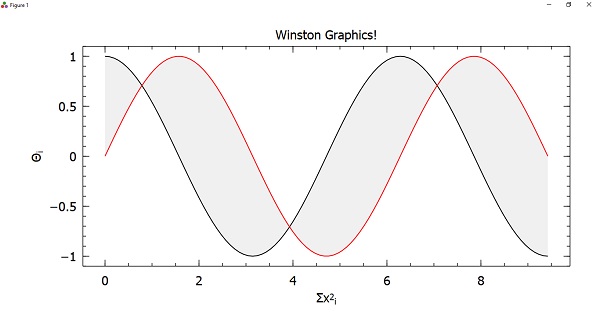
Data Visualization
Data visualization may be defined as the presentation of data in a variety of graphical as well as pictorial formats such as pie and bar charts.
Gadfly
Gadfly is a powerful Julia package for data visualization and an implementation of the grammar of graphics style. It is based on the same principal as ggplot2 in R. For using it, we need to first add it with the help of Julia package manager.
Example
To use Gadfly, we first need to use RDatasets package so that we can get some datasets to work with. In this example, we will be using iris dataset −
julia> using Gadflyjulia> using RDatasetsjulia> iris = dataset("datasets", "iris");julia> first(iris,10)105 DataFrame Row SepalLength SepalWidth PetalLength PetalWidth Species Float64 Float64 Float64 Float64 Cat 1 5.1 3.5 1.4 0.2 setosa 2 4.9 3.0 1.4 0.2 setosa 3 4.7 3.2 1.3 0.2 setosa 4 4.6 3.1 1.5 0.2 setosa 5 5.0 3.6 1.4 0.2 setosa 6 5.4 3.9 1.7 0.4 setosa 7 4.6 3.4 1.4 0.3 setosa 8 5.0 3.4 1.5 0.2 setosa 9 4.4 2.9 1.4 0.2 setosa 10 4.9 3.1 1.5 0.1 setosa Now let us plot a scatter plot. We will be using the variables namely SepalLength and SepalWidth. For this, we need to set the geometry element using Geom.point as follows −
julia> Gadfly.plot(iris, x = :SepalLength, y = :SepalWidth, Geom.point)

Similarly we can add some more geometries like geom.line to produce more layers in the plot −
julia> Gadfly.plot(iris, x = :SepalLength, y = :SepalWidth, Geom.point, Geom.line)
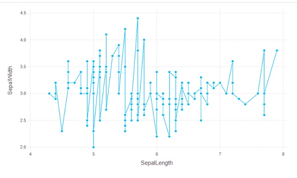
We can also set the color of keyword argument as follows −
julia> Gadfly.plot(iris, x = :SepalLength, y = :SepalWidth, color = :Species, Geom.point)
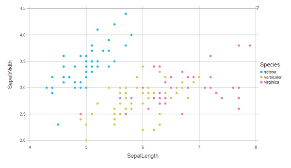
Compose
Compose is a declarative vector graphics system. It is also written by Daniel Jones as a part of the Gadfly system. In Compose, the graphics are defined using a tree structure and the primitives can be classified as follows −
Context − It represents an internal node.
Form − It represents a leaf node which defines some geometry such as a circle or line.
Property − It represents a leaf node that modifies how its parents subtree is drawn. For example, fill color and line width.
Compose(x,y) − It returns a new tree rooted at x and with y attached as child.
Example
The below example will draw a simple image −
julia> using Composejulia> composition = compose(compose(context(), rectangle()), fill("tomato"))julia> draw(SVG("simple.svg", 6cm, 6cm), composition)
Now let us form more complex trees by grouping subtrees with brackets −
julia> composition = compose(context(), (context(), circle(), fill("bisque")), (context(), rectangle(), fill("tomato")))julia> composition |> SVG("simple2.svg")
Graphics Engines
In this section, we shall discuss various graphic engines used in Julia.
PyPlot
PyPlot, arose from the previous development of the PyCall module, provides a Julia interface to the Matplotlib plotting library from Python. It uses the PyCall package to call Matplotlib directly from Julia. To work with PytPlot, we need to do the following setup −
julia> using Pkgjulia> pkg"up; add PyPlot Conda"julia> using Condajulia> Conda.add("matplotlib")Once you are done with this setup, you can simply import PyPlot by using PyPlot command. It will let you make calling functions in matplotlib.pyplot.
Example
This example, from PyPlot documentation, will create a sinusoidally modulated sinusoid −
julia> using PyPlotjulia> x = range(0; stop=2*pi, length=500);julia> y = sin.(3 * x + 4 * cos.(2 * x));julia> plot(x, y, color="blue", linewidth=1.0, linestyle="--")1-element Array{PyCall.PyObject,1}:PyObject <matplotlib.lines.Line2D object at 0x00000000323405E0>julia> title("A sinusoidally modulated sinusoid")PyObject Text(0.5, 1.0, 'A sinusoidally modulated sinusoid')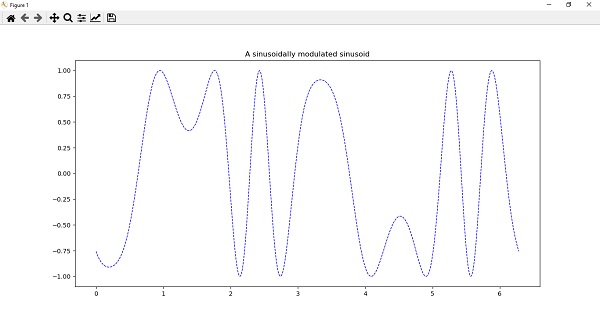
The PyPlot package can also be used for 3d plotting and for this it can import functions from Matplotlibs mplot3d toolkit. We can create 3d plots directly also by calling some corresponding methods such as bar3d, plot_surface, plot3d, etc., of Axes3d.
For example, we can plot a random surface mesh as follows −
julia> surf(rand(20,30))PyObject <mpl_toolkits.mplot3d.art3d.Poly3DCollection object at 0x00000000019BD550>
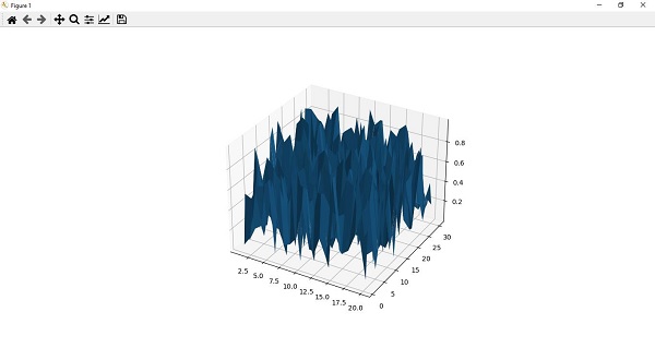
Gaston
Gaston is another useful package for plotting. This plotting package provides an interface to gnuplot.
Some of the features of Gaston are as follows −
It can plot using graphical windows, and with mouse interaction, it can keep multiple plots active at one time.
It can plot directly to the REPL.
It can also plot in Jupyter and Juno.
It supports popular 2-dimensional plots such as stem, step, histograms, etc.
It also supports popular 3-dimensional plots such as surface, contour, and heatmap.
It takes around five seconds to load package, plot, and save to pdf.
Example
A simple 2-D plot with the help of Gaston is shown below −
julia> x = 0:0.01:10.0:0.01:1.0julia> plot(x, sin.(2*5*t))
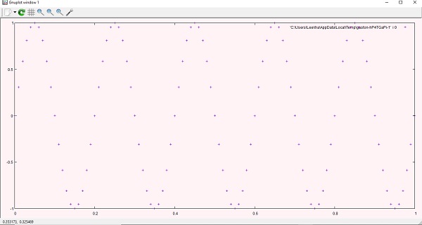
Now, we can add another curve as follows −
julia> plot!(x, cos.(2*5*t))
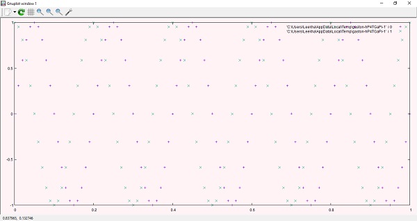
PyPlot can also be used to plot 3-d plots. Example is given below:julia> a = b = -10:0.30:10-10.0:0.3:9.8julia> surf(a, b, (a,b)->sin.(sqrt.(a.*a+b.*b))./sqrt.(a.*a+b.*b), title="Sombrero", plotstyle="pm3d")
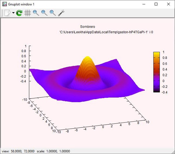
PGF Plots
PGFPlots, unlike Gaston, is relatively a new package for plotting. This plotting package uses the pgfplots LaTex routines to produce the plots. It can easily integrate with IJulia, outputting SVG images to notebook. To work with it, we need to install the following dependencies −
Pdf2svg, which is required by TikzPictures.
Pgfplots, which you can install using latex package manager.
GNUPlot, which you need to plot contours
Once you are done with these installations, you are ready to use PGFPlots.
In this example, we will be generating multiple curves on the same axis and assign their legend entries in LaTex format −
julia> using PGFPlotsjulia> R = Axis( [ Plots.Linear(x->sin(3x)*exp(-0.3x), (0,8), legendentry = L"$\sin(3x)*exp(-0.3x)$"), Plots.Linear(x->sqrt(x)/(1+x^2), (0,8), legendentry = L"$\sqrt{2x}/(1+x^2)$") ]); julia> save("Plot_LinearPGF.svg", R);Julia Programming - Networking
Sockets and Servers
To deal with streaming I/O objects such as pipes, TCP sockets, terminals, etc., we need a rich interface which is provided by Julia. This Julia interface is provided to the programmer in synchronous manner despite the fact that it is presented asynchronously at system level.
The advantage is that the programmer does not need to think about the underlying asynchronous operations. Before getting deep into this, we should know the concept of well-known ports.
Well-known ports
The concept of well-known ports and networked services on them was introduced in early 1980s by Berkeley development. It was first introduced to Unix. The basic idea behind this was −
A particular network service should associate with a particular port number.
And the network packet should be sent tagged with that port number.
Some of the well-known ports are as follows −
Port 21-file transfer protocol
Port 22-SSH
Port 25-sendmail
Port 80-web servers to deliver HTTP content
Port 3306-used commonly by MySQL database
Port 28017-used commonly by MongoDB Server
Port 6379- Stores Redis key-value
Julias UDP and TCP sockets
The internet protocol (IP) specified following two types of sockets −
Unreliable
The concept of unreliable socket rests in the fact that some requests which if not serviced, will be ignored, and retired. Example, requesting the network time from NNTP server. All these kinds of sockets are connectionless and operating via UDP (User Datagram Protocol).
Reliable
The concept of reliable sockets is opposite to unreliable sockets. They are connection full and operate via TCP (Transmission Control Protocol).
Julia supports both these sockets (UDP and TCP) and the source code is provided in socket.jl and streams.jl base modules.
Example
In the example given below, we will be creating a simple server involving TCP sockets −
julia> using Socketsjulia> @async begin server = listen(ip"127.0.0.1",2000) while true sock = accept(server) println("This is TCP server example\n") end endjulia> connect(2000)This is TCP server exampleNamed Pipes
Named pipes or UNIX domain sockets is a FIFO(First-in, First-out) stream and an extension to the traditional pipe mechanism on Unix and OS X. It is also available on Windows and has a specific pattern for the name prefix (\\.\pipe\). It is a communication channel which uses a special file.
Example
We can also create a named pipe server as given below −
julia> using Socketsjulia> @async begin server = listen("\\\\.\\pipe\\testsocket") while true sock = accept(server) println("This is a named pipe server example\n") end end julia> connect(2000)This is a named pipe server exampleA TCP web service
The functionality of a web browser is different from that of an echo server (which we developed earlier in this section). One important difference is that the web server should be able to return different file formats (JPEG, PNG, GIFs, TXT, etc.) and the browser should be able to distinguish between them.
Example
The following example will return a random quote as plain text from a text file −
julia> function web_server(sock::Integer) foo = open("/Users/Leekha/Desktop/Hello.txt"); header = """HTTP/1.1 200 OK Content-type: text/plain; charset=us-ascii """ ; wb = readlines(foo); close(foo); wn = length(wb); @async begin server = listen(sock) while true wi = rand(1:wn) ws = chomp(wb[wi]) sock = accept(server) println(header*ws) end end endweb_server (generic function with 1 method)julia> web_server(8080)Task (runnable) @0x0000000014bae570julia> conn = connect(8080)HTTP/1.1 200 OKContent-type: text/plain; charset=us-asciiHello, This is TutorialspointTCPSocket(Base.Libc.WindowsRawSocket(0x00000000000003f8) open, 0 bytes waiting)The Julia Web Group
The web browsers are mainly built with the property to respond to the request issued for a browser. Here we will discuss how we can interact with the Web through HTTP requests (for getting as well as posting data to the web).
First, we need to import the Requests.jl package as follows −
Pkg.add(Requests)
Next, import the necessary modules namely get and post as follows −
import Requests: get, post
Use GET request to request data from a specified web browser as follows −
get(url of the website)
If you want to request from a specified web page inside the website, use the query parameter as follows −
get(url of the website; query = Dict(title=>pagenumber/page name))
We can also set the timeouts for the GET request as follows −
get(url of the website; timeout = 0.2)
We can use the below command to avoid getting your request repeatedly redirected to different websites −
get(url of the website; max_redirects = 2)
Using the below command prevents the site from redirecting your GET request −
get(url of tcommand he website; allow_redirects = false)
To send the post request, we have to use the below command −
post(url of the website)
Using the below command, we can send data to web browser through the POST request −
post(url of the website, data = Data to be sent)
Let us see how we can send data such as session cookies to web browser through the POST request −
post(url of the website, cookies = Dict(sessionkey=> key)
Files can also be sent as follows −
file = "book.jl"post("url of the website"; files = [FileParam(file), "text/julia","file_name", "file_name.jl"])WebSockets
We are familiar with the method called AJAX (Asynchronous JavaScript and XML). The example for this method can be the process where we type in the search box and the server returns a set of suggestions and they change as the search term is refined. With this, it is clear that the overhead usage of HTTP protocols is very high.
Web Sockets, which combine the parts of UDP and TCP, are the way to overcome this problem. Hence, web sockets are message-based such as UDP and reliable as TCP. It uses normal HTTP/HTTPS ports, i.e., port 80 and port 443 respectively. They are ideal for vehicles for chat services. Julia provides a package named websockets.jl.
Messaging
Julia supports the following messaging methods −
Email is one of the oldest messaging methods. Email messaging can be done in two ways −
Sending e-mails − It happens on well-known port 25. Some other ports such as 465 and 587 can also be used for this purpose. SMTP (Simple Mail Transport Protocol) that consists of formulating a message the SMTP server can understand is used for sending emails. To:, From:, and Subject:, all together with the message should be deposited in the mail services outbound queue.
Receiving e-mails − It is a bit different from sending emails. It basically depends on POP (Post Office Protocol) or IMAP (Internet Message Access Protocol).
Example
Following code can be used to send emails −
using SMTPClientopt = SendOptions( isSSL = true, username = "g*****@gmail.com", passwd = "yourgmailpassword")body = IOBuffer( "Date: Fri, 25 Sep 2020 19:44:35 +0100\r\n" * "From: You <you@gmail.com>\r\n" * "To: me@test.com\r\n" * "Subject: Test_email\r\n" * "\r\n" * "Test Message\r\n")url = "smtps://smtp.gmail.com:465"rcpt = ["<me@gmail.com>", "<foo@gmail.com>"]from = "<you@gmail.com>"resp = send(url, rcpt, from, body, opt)
Apart from E-mail, there are other systems that send SMS textual information. One of them is Twitter. Julia provides a package named Twitter.jl to work with Twitter API. To work with Twitter on Julia, we need to authenticate. For authentication, we need to first create an application on dev.twitter.com. After setting up the application, we will be able to access our consumer_key, consumer_token, oauth_token, and oauth_secret.
using Twittertwitterauth("1234567nOtp...", "1234sES96S...", "45750-Hjas...", "Uonhjlmkmj...")If you want to say hello to all your Twitter followers, use the following code −
post_status_update("Hello")And if you want to search the tweets containing the hashtag say #TutorialsPoint, the function call will be as follows −
my_tweets = get_search_tweets("#TutorialsPoint")The Twitter API bydefault will return the 15 most recent tweets containing the above searched hastag.
Suppose if you want to return the most recent 50 tweets, you can pass the count as follows −
my_tweets_50 = get_search_tweets("#TutorialsPoint"; options = {"count" => "50"})DataFrame method can be defined as follows −
df_tweets = DataFrame(my_tweets_50)
Cloud Services
Julia offers the following cloud services −
The AWS.jl Package
The AWS.jl package is a Julia interface for Amazon Web Services. It replaces AWSCore.jl (provided low-level) and AWSSDK.jl (provided high-level) packages. The AWS.jl package −
Includes automated code generation to ensure all new AWS services are available.
Keeps the existing service up to date.
We can install this package with the following code −
julia> Pkg.add("AWS")AWS.jl package can be used with both low-level and high-level API requests. Following are the services supported −
EC2
S3
SQS
Auto Scaling
AWSEnv
The structure of AWSEnv is as follows −
type AWSEnv aws_id::String # AWS Access Key id aws_seckey::String # AWS Secret key for signing requests aws_token::String # AWS Security Token for temporary credentials region::String # region name ep_scheme::String # URL scheme: http or https ep_host::String # region endpoint (host) ep_path::String # region endpoint (path) sig_ver::Int # AWS signature version (2 or 4) timeout::Float64 # request timeout in seconds, Default is 0.0 dry_run::Bool # If true, no actual request will be made dbg::Bool # print request and raw response to screenend
Constructors
Following are the constructors in AWS −
AWSEnv(; id=AWS_ID, key=AWS_SECKEY, token=AWS_TOKEN, ec2_creds=false, scheme="https", region=AWS_REGION, ep="", sig_ver=4, timeout=0.0, dr=false, dbg=false)
Here,
AWS_ID and AWS_SECKEY both are initialized from env.
AWS_TOKEN − It is by default an empty string.
ec2_creds − It should be set to true to automatically retrieve temporary security credentials.
region − It should be set to one of the AWS region name strings.
ep − It can contain both a hostname and a pathname for an AWS endpoint.
sig_ver − It is signature version and must be set to 2 or 4.
Binary Dependencies
Following must be installed before using AWS −
libz
libxm2
The Google Cloud
The GoogleCloud.jl is the module that wraps GCP (Google Clous Platform) APIs with Julia.
Prerequisites
Following are some prerequisites for Google Cloud −
Create a Google account if you do not already have.
Need to sign in to the GCP console.
You need to create a new project. Click on the Project drop-down menu at the top of the page.
You need to first get the credentials from your GCP credentials page, that are associated with your project, as a JSON file.
Save this json file to your local computer.
Interacting with the API from Julia
First install the GoogleCloud,jl package as follows −
Pkg.add(GoogleCloud)using GoogleCloud
Now we need to load the service account credentials obtained from Google account −
creds = GoogleCredentials(expanduser("put here address of .json file"))Create a session as follows −
session = GoogleSession(creds, ["devstorage.full_control"])
By using set_session, set the default session of an API −
set_session!(storage, session)
You can list all the buckets in your existing project as shown below −
bkts = storage(:Bucket, :list)for item in bkts display(item) println()end
Now let us create a new bucket named foo_bkt as follows −
storage(:Bucket, :insert; data=Dict(:name => "foo_bkt"))bkts = storage(:Bucket, :list)for item in bkts display(item) println()end
You can list all the objects that are in foo_bkt −
storage(:Object, :list, "foo_bkt")
You can delete the bucket as follows −
storage(:Bucket, :delete, "foo_bkt")bkts = storage(:Bucket, :list)for item in bkts display(item) println()end
Julia Programming - Databases
Following are the four mechanisms for interfacing with a particular database system −
First method of accessing a database is by using the set of routines in an API (Application Program Interface). In this method, the DBMS will be bundled as a set of query and maintenance utilities. These utilities will communicate with the running database through a shared library which further will be exposed to the user as a set of routines in an API.
Second method is via an intermediate abstract layer. This abstract layer will communicate with the database API via a driver. Some example of such drivers are ODBC, JDBC, and Database Interface (DBI).
Third approach is to use Python module for a specific database system. PyCall package will be used to call routines in the Python module. It will also handle the interchange of datatypes between Python and Julia.
The fourth method is sending messages to the database. RESTful is the most common messaging protocol.
Julia Database APIs
Julia provides several APIs to communicate with various database providers.
MySQL
MySQL.jl is the package to access MySQL from Julia programming language.
Use the following code to install the master version of MySQL API −
Pkg.clone("https://github.com/JuliaComputing/MySQL.jl")Example
To access MySQL API, we need to first connect to the MySQL server which can be done with the help of following code −`
using MySQLcon = mysql_connect(HOST, USER, PASSWD, DBNAME)
To work with database, use the following code snippet to create a table −
command = """CREATE TABLE Employee ( ID INT NOT NULL AUTO_INCREMENT, Name VARCHAR(255), Salary FLOAT, JoinDate DATE, LastLogin DATETIME, LunchTime TIME, PRIMARY KEY (ID) );"""response = mysql_query(con, command)if (response == 0) println("Create table succeeded.")else println("Create table failed.")endWe can use the following command to obtain the SELECT query result as dataframe −
command = """SELECT * FROM Employee;"""dframe = execute_query(con, command)
We can use the following command to obtain the SELECT query result as Julia Array −
command = """SELECT * FROM Employee;"""retarr = mysql_execute_query(con, command, opformat=MYSQL_ARRAY)
We can use the following command to obtain the SELECT query result as Julia Array with each row as a tuple −
command = """SELECT * FROM Employee;"""retarr = mysql_execute_query(con, command, opformat=MYSQL_TUPLES)
We can execute a multi query as follows −
command = """INSERT INTO Employee (Name) VALUES ('');UPDATE Employee SET LunchTime = '15:00:00' WHERE LENGTH(Name) > 5;"""data = mysql_execute_query(con, command)We can get dataframes by using prepared statements as follows −
command = """SELECT * FROM Employee;"""stmt = mysql_stmt_init(con)if (stmt == C_NULL) error("Error in initialization of statement.")endresponse = mysql_stmt_prepare(stmt, command)mysql_display_error(con, response != 0, "Error occured while preparing statement for query \"$command\"") dframe = mysql_stmt_result_to_dataframe(stmt)mysql_stmt_close(stmt)Use the following command to close the connection −
mysql_disconnect(con)
JDBC
JDBC.jl is Julia interface to Java database drivers. The package JDBC.jl enables us the use of Java JDBC drivers to access databases from within Julia programming language.
To start working with it, we need to first add the database driver jar file to the classpath and then initialize the JVM as follows −
using JDBCJavaCall.addClassPath("path of .jar file") # add the path of your .jar fileJDBC.init()Example
The JDBC API in Julia is similar to Java JDBC driver. To connect with a database, we need to follow similar steps as shown below −
conn = DriverManager.getConnection("jdbc:gl:test/juliatest")stmt = createStatement(conn)rs = executeQuery(stmt, "select * from mytable") for r in rs println(getInt(r, 1), getString(r,"NAME"))endIf you want to get each row as a Julia tuple, use JDBCRowIterator to iterate over the result set. Note that if the values are declared to be nullable in the database, they will be of nullable in tuples also.
for r in JDBCRowIterator(rs) println(r)end
Updating the table
Use PrepareStatement to do insert and update. It has setter functions defined for different types corresponding to the getter functions −
ppstmt = prepareStatement(conn, "insert into mytable values (?, ?)")setInt(ppstmt, 1,10)setString(ppstmt, 2,"TEN")executeUpdate(ppstmt)
Running stored procedures
Use CallableStatement to run the stored procedure −
cstmt = JDBC.prepareCall(conn, "CALL SYSCS_UTIL.SYSCS_SET_DATABASE_PROPERTY(?, ?)")setString(cstmt, 1, "gl.locks.deadlockTimeout")setString(cstmt, 2, "10")execute(cstmt)
Metadata
In order to get an array of (column_name, column_type) tuples, we need to Pass the JResultSet object from executeQuery to getTableMetaData as follows −
conn = DriverManager.getConnection("jdbc:gl:test/juliatest")stmt = createStatement(conn)rs = executeQuery(stmt, "select * from mytable")metadata = getTableMetaData(rs)Use the following command to close the connection −
close(conn)
Executing a query
For executing a query, we need a cursor first. Once obtained a cursor you can run execute! command on the cursor as follows −
csr = cursor(conn)execute!(csr, "insert into ptable (pvalue) values (3.14);")execute!(csr, "select * from gltable;")
Iterating over the rows
We need to call rows on the cursor to iterate over the rows −
rs = rows(csr)for row in rsend
Use the following command to close the cursor call −
close(csr)
ODBC
ODBC.jl is a package which provides us a Julia ODBC API interface. It is implemented by various ODBC driver managers. We can install it as follows −
julia> Pkg.add(ODBC)
Installing ODBC Driver
Use the command below to install an ODBC driver −
ODBC.adddriver("name of driver", "full, absolute path to driver shared library"; kw...)We need to pass −
The name of the driver
The full and absolute path to the driver shared library
And any additional keyword arguments which will be included as KEY=VALUE pairs in the .ini config files.
Enabling Connections
After installing the drivers, we can do the following for enabling connections −
Setup a DSN, via ODBC.adddsn("dsn name", "driver name"; kw...)
Connecting directly by using a full connection string like ODBC.Connection(connection_string)
Executing Queries
Following are two paths to execute queries −
DBInterface.execute(conn, sql, params) − It will directly execute a SQL query and after that will return a Cursor for any resultset.
stmt = DBInterface.prepare(conn, sql); DBInterface.execute(stmt, params) − It will first prepare a SQL statement and then execute. The execution can be done perhaps multiple times with different parameters.
SQLite
SQLlite is a fast, flexible delimited file reader and writer for Julia programming language. This package is registered in METADATA.jl hence can be installed by using the following command −
julia> Pkg.add("SQLite")We will discuss two important and useful functions used in SQLite along with the example −
SQLite.DB(file::AbstractString) − This function requires the file string argument as the name of a pre-defined SQLite database to be opened. If the file does not exit, it will create a database.
Example
julia> using SQLitejulia> db = SQLite.DB("Chinook_Sqlite.sqlite")Here we are using a sample database Chinook available for SQLite, SQL Server, MySQL, etc.
SQLite.query(db::SQLite.DB, sql::String, values=[]) − This function returns the result, if any, after executing the prepared sql statement in the context of db.
Example
julia> SQLite.query(db, "SELECT * FROM Genre WHERE regexp('e[trs]', Name)")6x2 ResultSet| Row | "GenreId" | "Name" ||-----|-----------|----------------------|| 1 | 3 | "Metal" || 2 | 4 | "Alternative & Punk" || 3 | 6 | "Blues" || 4 | 13 | "Heavy Metal" || 5 | 23 | "Alternative" || 6 | 25 | "Opera" |PostgreSQL
PostgreSQL.jl is the PostgreSQL DBI driver. It is an interface to PostgreSQL from Julia programming language. It obeys the DBI.jl protocol for working and uses the C PostgreeSQL API (libpq).
Lets understand its usage with the help of following code −
using DBIusing PostgreSQLconn = connect(Postgres, "localhost", "username", "password", "dbname", 5432)stmt = prepare(conn, "SELECT 1::bigint, 2.0::double precision, 'foo'::character varying, " * "'foo'::character(10);")result = execute(stmt)for row in resultendfinish(stmt)disconnect(conn)
To use PostgreSQL we need to fulfill the following binary requirements −
DBI.jl
DataFrames.jl >= v0.5.7
DataArrays.jl >= v0.1.2
libpq shared library (comes with a standard PostgreSQL client installation)
julia 0.3 or higher
Hive
Hive.jl is a client for distributed SQL engine. It provides a HiveServer2, for example: Hive, Spark, SQL, Impala.
Connection
To connect to the server, we need to create an instance of the HiveSession as follows −
session = HiveSession()
It can also be connected by specifying the hostname and the port number as follows −
session = HiveSession(localhost,10000)
The default implementation as above will authenticates with the same user-id as that of the shell. We can override it as follows −
session = HiveSession("localhost", 10000, HiveAuthSASLPlain("uid", "pwd", "zid"))Executing the queries
We can execute DML, DDL, SET, etc., statements as we can see in the example below −
crs = execute(session, "select * from mytable where formid < 1001"; async=true, config=Dict())while !isready(crs) println("waiting...") sleep(10)endcrs = result(crs)Other Packages
DBAPI is a new database interface proposal, inspired by Pythons DB API 2.0, that defies an abstract interface for database drivers in Julia. This module contains the following −
Abstract types
Abstract required functions which throw a NotImplementedError by default
Abstract optional functions which throw a NotSupportedError by default
To use this API, the database drivers must import this module, subtype its types, and create methods for its functions.
DBPrf is a Julia database which is maintained by JuliaDB. You see its usage below −
The user can provide input in two ways −
Command-Line mode
$ julia DBPerf.jl <Database_Driver_1.jl> <Database_Driver_2.jl> ....... <Database_Driver_N.jl> <DBMS>
Here, Database_Driver.jl can be of the following types −
ODBC.jl
JDBC.jl
PostgreSQL.jl
MySQL.jl
Mongo.jl
SQLite.jl
DBMS filed is applicable only if we are using JDBC.jl.
The database can be either Oracle or MySQL.
Example
DBPerf.jl ODBC.jl JDBC.jl MySql
Executing from Julia Prompt
julia> include("DBPerf.jl")julia> DBPerf(<Database_Driver_1.jl>, <Database_Driver_2.jl>, ....... <Database_Driver_N.jl>, <DBMS>)Example
DBPerf(ODBC.jl, JDBC.jl, MySql)