MATLAB Simulink - Quick Guide

MATLAB Simulink - Introduction

Simulink is a simulation and model-based design environment for dynamic and embedded systems, which are integrated with MATLAB. Simulink was developed by a computer software company MathWorks.

It is a data flow graphical programming language tool for modelling, simulating and analysing multi-domain dynamic systems. It is basically a graphical block diagramming tool with a customisable set of block libraries.

Furthermore, it allows you to incorporate MATLAB algorithms into models as well as export the simulation results into MATLAB for further analysis.

Simulink supports the following −

System-level design.
Simulation.
Automatic code generation.
Testing and verification of embedded systems.

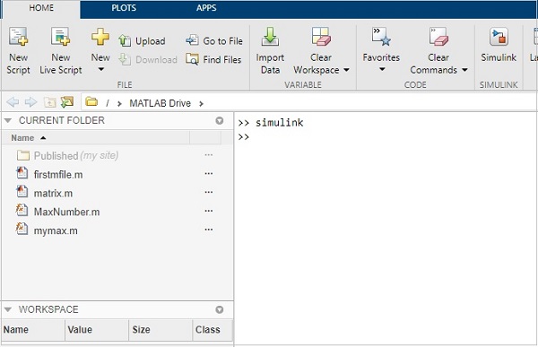
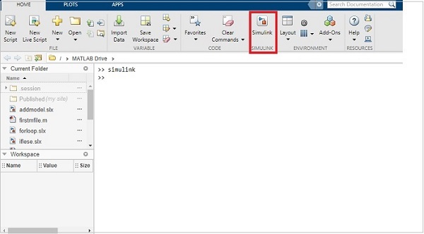
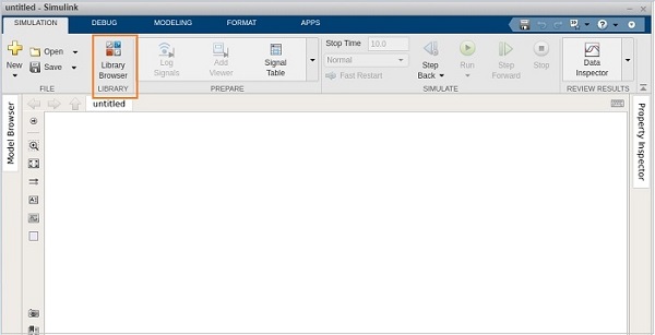
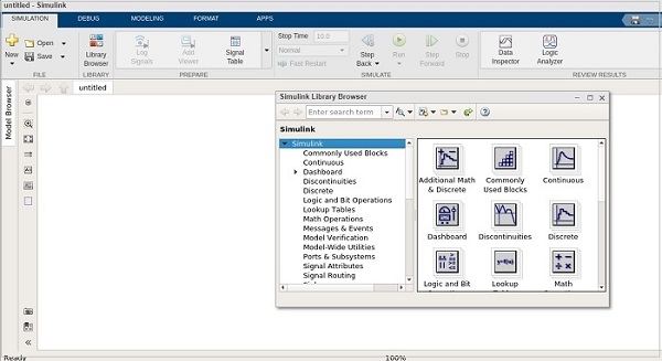
To get started with Simulink, type simulink in the command window as shown below −

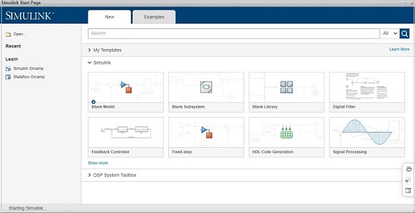
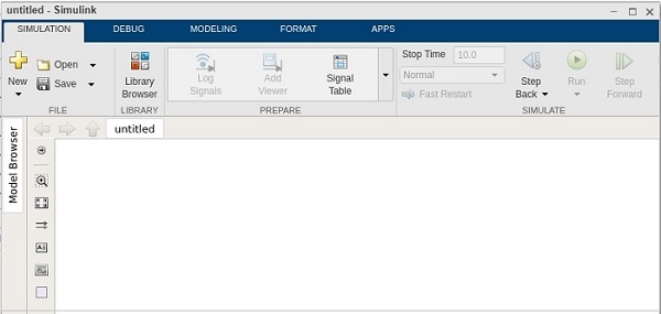
It will open the Simulink page as shown below −

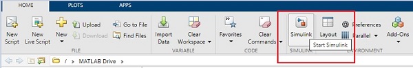
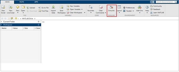
You can also make use of Simulink icon present in MATLAB to get started with Simulink −

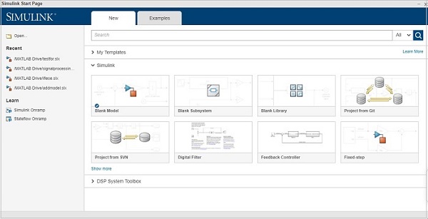
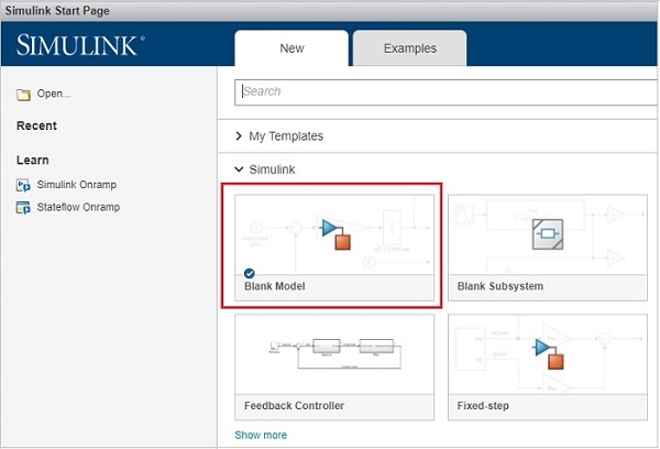
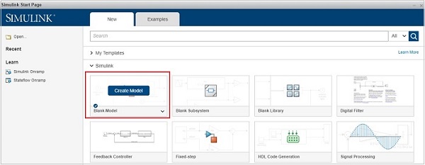
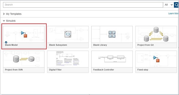
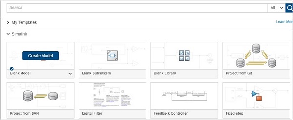
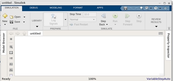
When you start Simulink, you are navigated to the start page as shown below

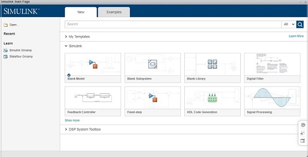
Here you can create your own model, and also make use of the existing templates.

Click on the Blank Model and you will get a Simulink library browser that can be used to create your own model.

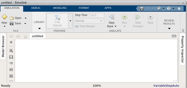
The screen for Blank model is as follows −

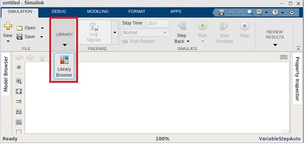
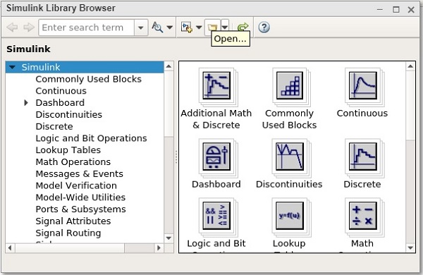
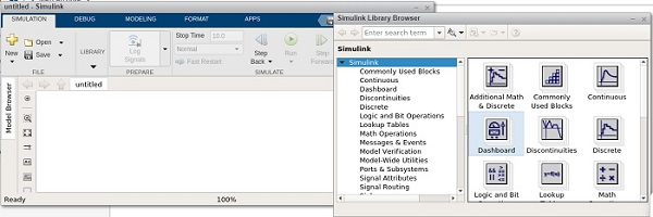
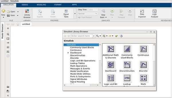
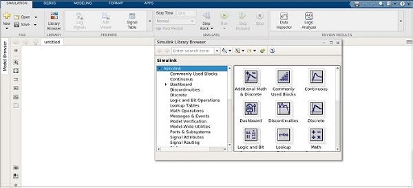
Click on Library and it will display you the Simulink library as shown below −

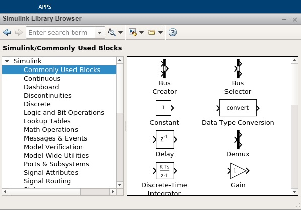
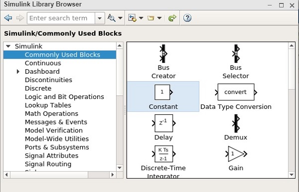
The Simulink library browsers is a collection of many libraries. It offers Commonly Used Blocks, Continuous, Dashboard, Logic and Bit Operation, Math Operations etc.

Besides that, you will get other library list like Control system toolbox, DSP system toolbox etc.

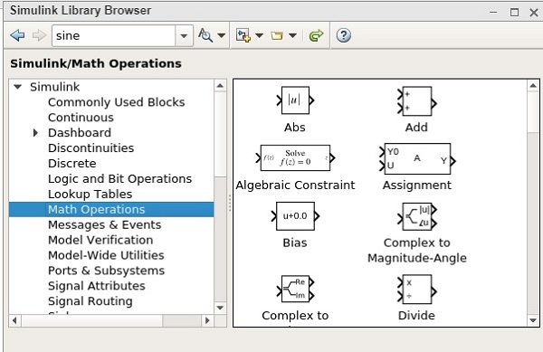
Here is an example of Math operations library list −

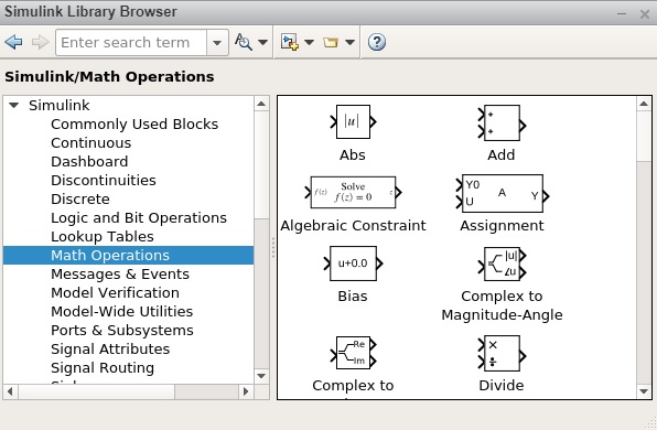
It has Abs, Add, Algebraic Constraint, Assignment etc. that you can make use in your model.

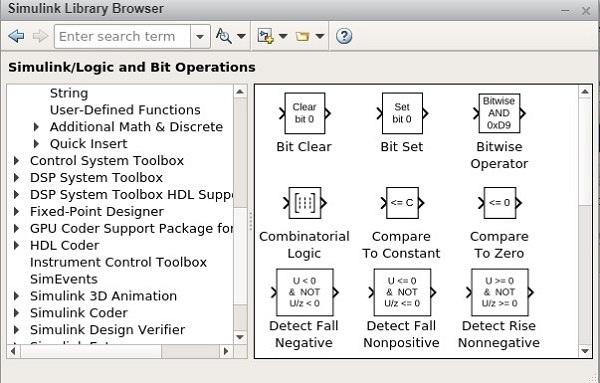
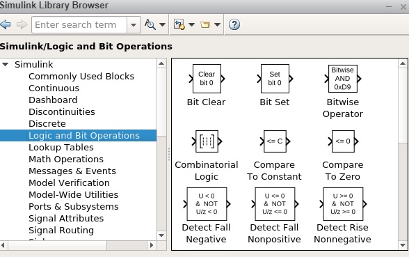
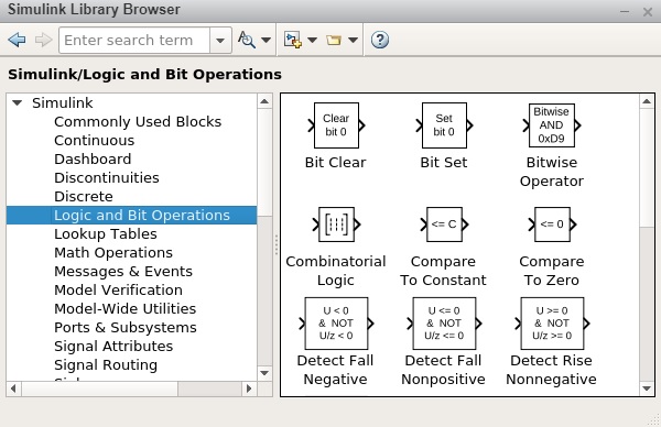
Given below is an example of Logic and Bit Operations −

MATLAB Simulink - Environment Setup

MATLAB simulink is a MATLAB product and to work with it, we need to download MATLAB.

The official website of matlab is https://www.mathworks.com/

The following page will appear on your screen −

To download MATLAB go to https://in.mathworks.com/downloads/ as shown below.

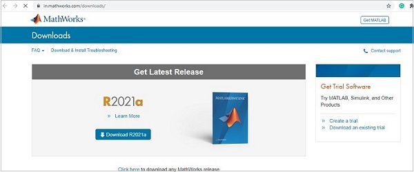
MATLAB is not free to download and you need to pay for the licensed copy. Later on you can download it.

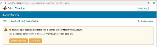
A free trial version is available for which you have to create a login for your respective account. Once an account is created, they allow you to download MATLAB and also an online version for a trial of 30 days’ license.

Once you are done with the creating a login from their website, download MATLAB and install on your system. Then, start MATLAB or you can also make use of their online version.

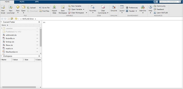
Simulink comes in-built with MATLAB. Once you install MATLAB, you will get Simulink as shown below −

MATLAB Simulink - Starting Simulink

In this chapter, we will understand about using Simulink to build models.

Here is a MATLAB display −

You can start Simulink by using simulink command in the MATLAB command window as shown below −

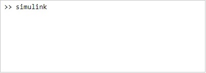
Click on enter to open the Simulink startup page as shown below −

You can also open Simulink from MATLAB interface directly by clicking on Simulink icon as shown below −

When you click on the Simulink icon, it will take you to a Simulink startup page, as shown below −

The startup page has a blank model, subsystem, library to start the model from scratch.

There are also some built-in templates that can help the users to start with.

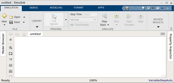
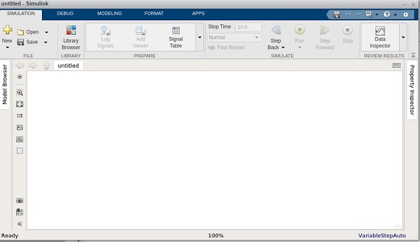
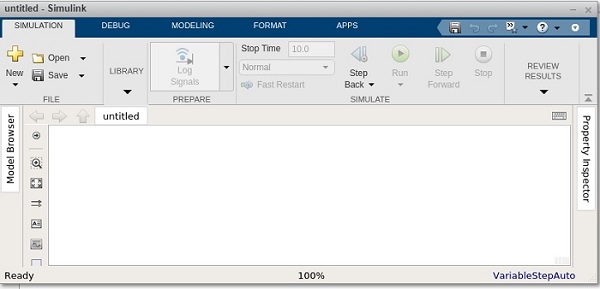
To create a model, the user can click on blank model and it will display a page as shown below −

Click on Save to save your model. The blocks to build your model are available inside the Simulink library browser.

Click on library browser as shown below −

The library browser has a list of all types of libraries with different blocks as shown below −

Libraries in Simulink

Let us understand some of the commonly used libraries in Simulink.

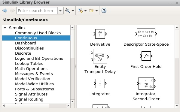
Continuous

A continuous blocks library gives you blocks related to derivatives and integrations. The list of blocks are as follows −

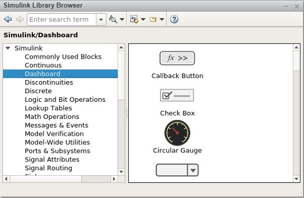
Dashboard

With Dashboard, you will get controls and indicator blocks that help to interact with simulations. The following screen will appear on your computer −

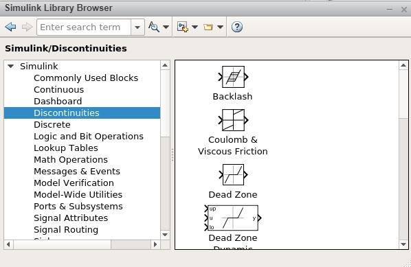
Discontinuities

Here, you will get a list of discontinuous functions blocks as displayed below −

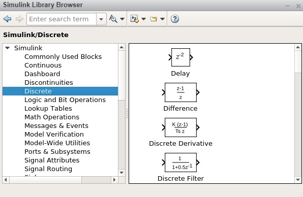
Discrete

Here, you will get time relation function blocks as shown below −

Logic and Bit Operations

In this category, you will get all logical and relational type blocks as displayed below −

Lookup Tables

You will all the sine, cosine function blocks as shown below −

Math Operations

All mathematical operations like Add, Absolute, divide, subtract are available. The list is as follows −

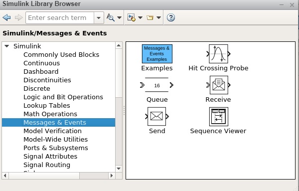
Messages and Events

This block has all the message/communication related functions as shown below −

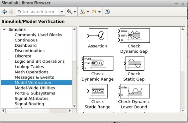
Model Verification

The blocks present here helps to self-verify models, such as Check Input Resolution. The following screen will appear on your computer −

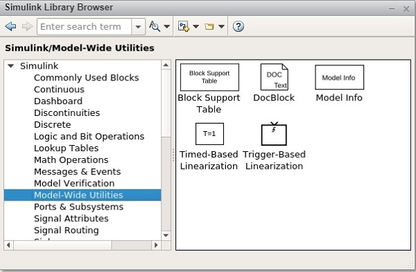
Model-Wide Utilities

This gives you blocks like Model info, Block Support Table etc. The following screen will appear on your computer −

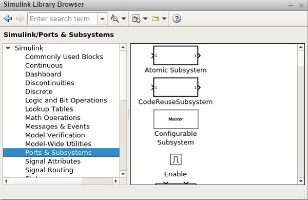
Ports and Subsystems

You will get blocks like a subsystem, switch case, enable etc. The list is displayed below −

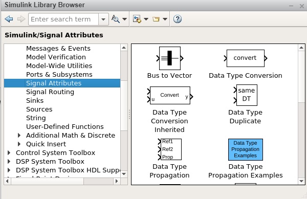
Signal Attributes

Modify the signal attribute blocks such as Data Type Conversion. The following screen will appear on your computer −

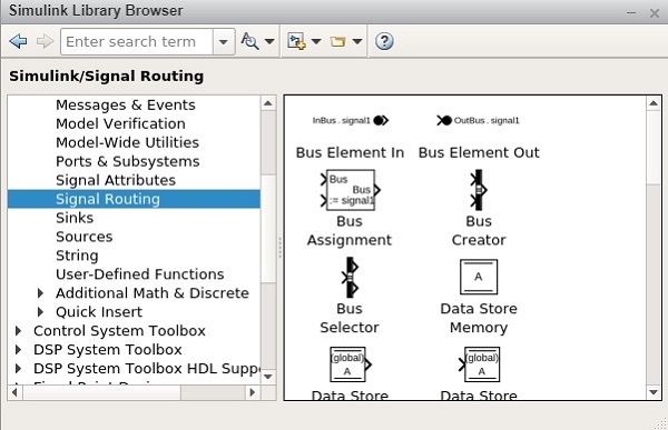
Signal Routing

The blocks in this category is used to route signal blocks such as bus creator, switch etc.The following screen will appear on your computer −

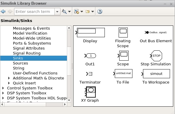
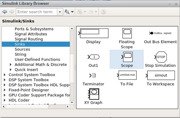
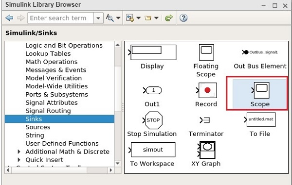
Sinks

The blocks in this category help to display or export signal data blocks such as Scope andTo Workspace. The following screen will appear on your computer −

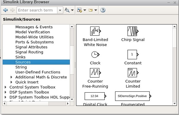
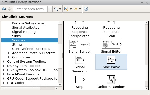
Sources

It helps to generate or import data blocks. For example, sine wave. The following screen will appear on your computer −

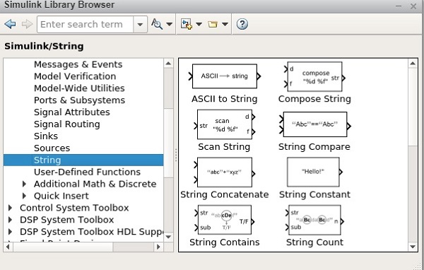
String

This category has string related blocks as shown below −

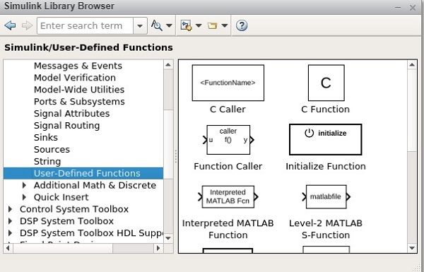
User Defined functions

Custom function blocks such as MATLAB Function, MATLAB System, Simulink Function, and Initialize Function. The following screen will appear on your computer −

MATLAB Simulink - Blocks

In this chapter, we will learn about one of the basic elements in Simulink. These are termed as blocks.

Blocks in Simulink helps to create models. You can make use of a Simulink library browser that has different types of blocks for creating a model.

First, open a blank model. The display will be as shown below −

You can save your model by clicking on the Save button. Hence, your changes will be saved successfully. Now, open the library browser to get the blocks into your model canvas.

The two ways to select the blocks are as follows −

Using Simulink browser library.
Searching for block inside model canvas.

Simulink browser library

Open the Simulink library browser as shown below −

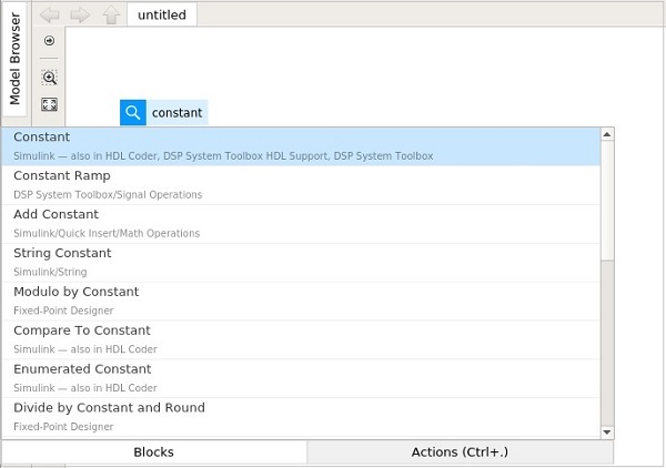
If you looking for a specific block and don’t know which library, you can search for it inside the search block which is available as shown below −

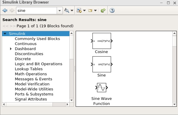
Here, we got all the blocks related to Sine. You can also go inside the library and pick your block.

Add block, Product block etc. The display will be as shown below −

To bring the block inside your model, you can select the block and drag it inside your model, as shown below −

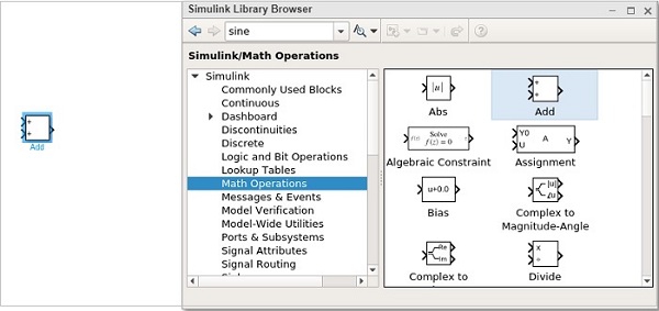
Another way is to right click the block and add to your current model.

An example for the same is given below −

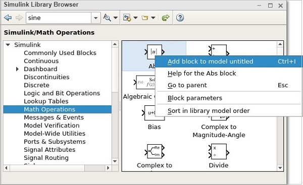
We have not saved our model. Hence, it comes as untitled. Now, you can add to the model untitled. The block will be seen inside your mode.

Searching for block inside model canvas

Another way to add blocks to your model is to click inside the model and type the name of the block. It will search in the library browser and list all the model as per what you have typed.

An example for the same is given below −

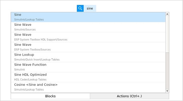
We have typed Sine and it displays all the blocks related to sine.

MATLAB Simulink - Lines

In the previous chapter, we learnt about the different types of blocks which are available with Simulink library. In this chapter, we are going to understand about lines.

Lines are used to connect the blocks with an arrow. Each block will have its own input and output connector. The communication between the blocks will take place with the help of lines.

Let us understand the same with an example. Select a blank model from Simulink page as shown below −

It will open a blank model workspace as shown below −

Click on Simulink Library browser to drag some blocks in the model workspace.

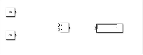
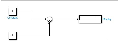
Consider that in the model, we want to add two given numbers. So let us pick the Add block, the display block and the constant block.

The constant block has one output connector, the Add block has two input connectors and the display block has one input connector respectively. You can drag the link from one output to another input as shown below.

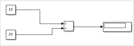
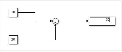
Here, we have two constants with values 10 and 20. They are connected to the add block with lines. The add block is connected to display with a line.

When the lines are connected, the display is as follows −

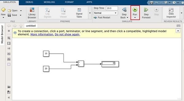
Now click on Run to see the result in the display block. It will add 10 + 20 to give the result as 30 in the display block.

MATLAB Simulink - Build & Simulate Model

We have seen the Simulink library browser and the blocks available in the library list. In this chapter, we are going to use the blocks to build a simple sine wave model.

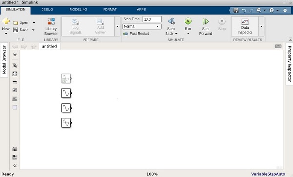
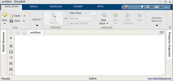
Open Simulink and click on blank model as shown below −

The blank model will open a blank popup window as shown below −

Now, open the Simulink Library browser so that we can select the blocks.

The following screen will appear on your computer

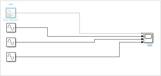
To move the sine wave to your model, select the block and drag it inside your model workspace. We want to display the sine wave and here, we have taken four sign wave in our model workspace as shown below −

Now we want to display the output of the signal, so let us use a Scope block from sinks library as shown below −

Now select and drag the Scope block inside your model workspace.

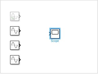
The sine wave has one output and the scope block has one input. We have four sine waves displayed. We have to change the parameters of scope block to take four inputs.

Right click on scope block and click on Block Parameters and it will display the screen as shown below −

Go to settings icon and change the input parameter from 1 to 4 as shown below −

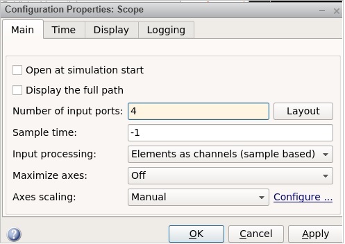
Click on Apply to save the changes.

Let us now connect the sine wave to the scope block with arrows as shown below −

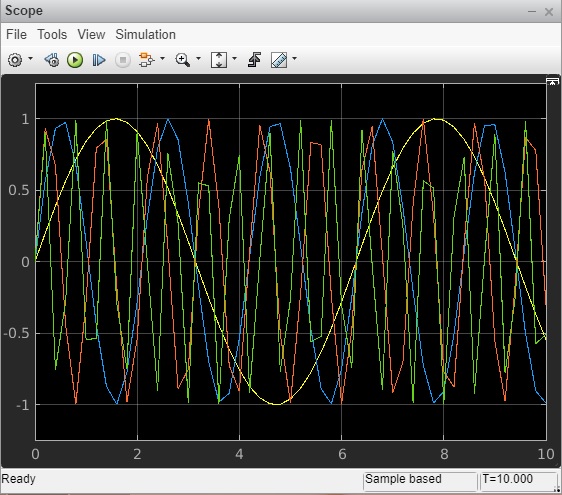
We would like to change the frequency of each sine wave to a different one, so that we get a signal graph of different frequencies.

So right click on sine wave and open the Sine wave block parameters as shown below −

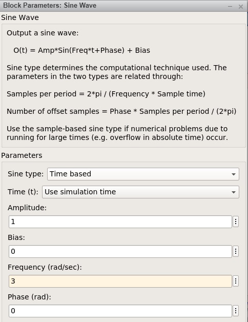
We are going to keep the amplitude as 1 for all sine waves and the frequency of the first sine wave is 1, second one is 3, third one is 6 and the last one is 10.

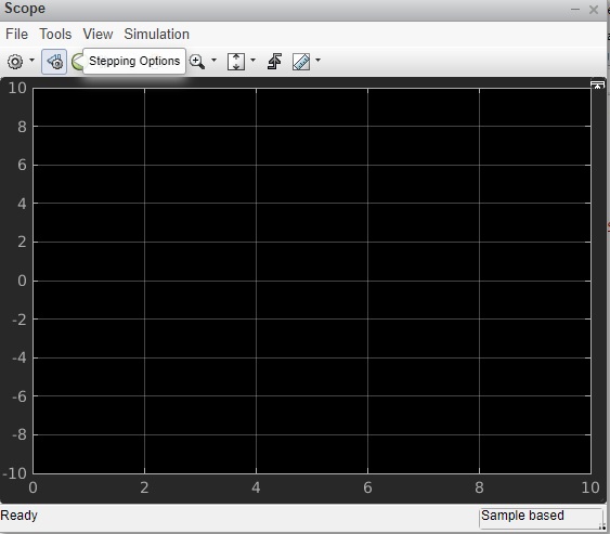
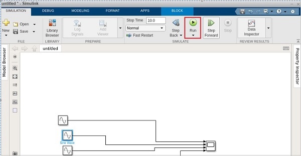
Click on the Run button as shown below to see the sine wave.

Open the scope block parameters to see the sine wave as shown below.

MATLAB Simulink - Signals Processing

In this chapter, we will understand the signals generation in Simulink. To start with, select a blank model from Simulink page and open Simulink browser library as shown below −

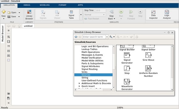
In sources library, you will get a signal generator symbol. It will help us to create different types of signals.

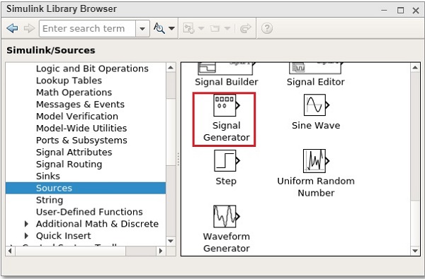
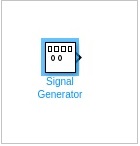
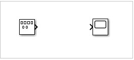
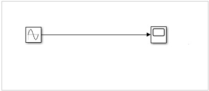
Select the Signal Generator and drag it to get inside the blank model as shown below −

To see the output of the signal generator, we need one more block called scope from sinks library as shown below −

Select the block and drag it to get inside the model.

Double click on signal generator or right click and select block parameters and it will display a screen as shown below −

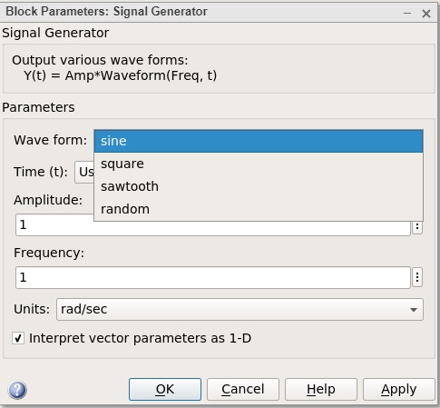
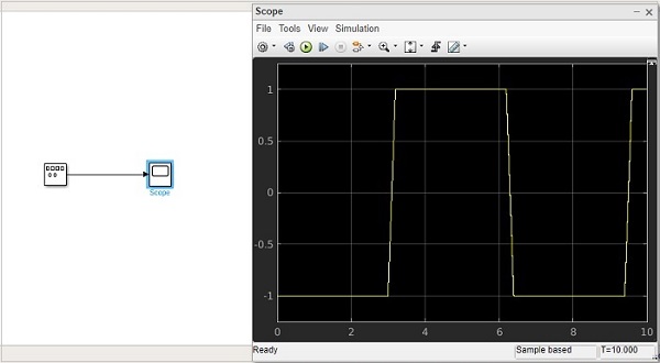
The signal generator can show waveforms like sine, square, sawtooth, random. We will select the square waveform. Let the amplitude and frequency be as 1. Click on OK to update the changes made.

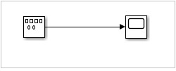
Now, connect the lines between signal generator and scope block as shown below −

Now click on Run button to see the square waveform as shown below −

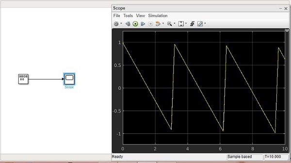
Let us now try the sawtooth wave form. Right click signal generator or double click and change the waveform to sawtooth.

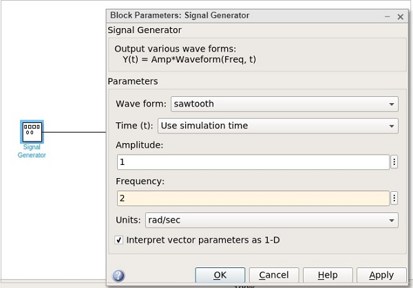
Let us change the frequency to 2. Click on OK to update the changes. Now run the model to see the changes as shown below −

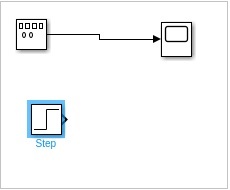
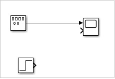
Let us now add some more signals to the above model. We will take the step signal from the sources library as shown below −

We just have one input for the scope block. Let us increase it to 2 inputs. Right click and open the block parameters.

Click on OK button to update the changes. Now, the scope block has 2 inputs as shown below −

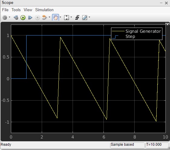
Connect the step input arrow with the scope arrow.

Now click on Run button to run the model.

You can add some more signals and test the same.

MATLAB Simulink - Adding Delay To Signals

We have learnt in the previous chapter about the different signal simulations. In this chapter, we will learn how to add delay to the signals.

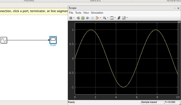
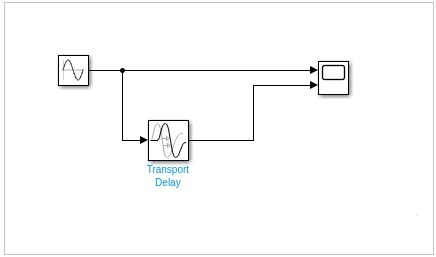
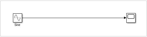
Let us take a blank model and add sine wave and scope block to it as shown below −

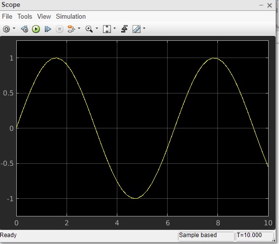
Let us now run the model to see the simulation in scope block. The sine wave is as shown below −

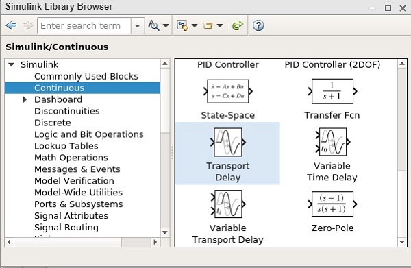
Let us now add delay for the sine wave. We will make use of transport delay block from continuous library as shown below −

Select the block and drag it in your model canvas. Now that we have the Transport delay in our model, right click on it and open block parameters as shown below −

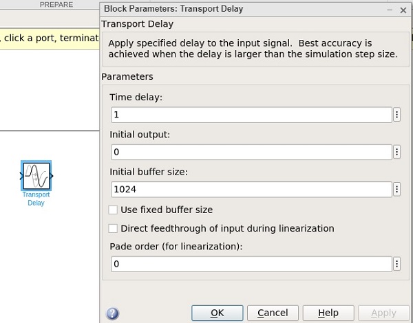
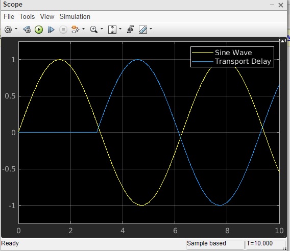
Let us change the time delay from 1 to 3. Make the changes and click on OK button.

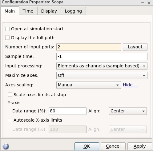
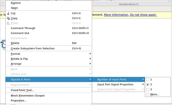
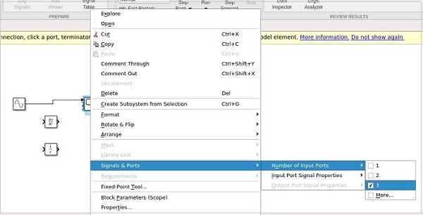
Now add one more input port to scope block. Right click on scope block and select the signals and ports. Select 2 for number of input ports as shown below −

Now connect the transport delay to sine wave and to scope as shown below

Now run the simulation to see a delay of 3 seconds to the sign wave. Right click scope block and select block parameters to see the display.

MATLAB Simulink - Mathematical Library

In this chapter, we will learn how to sum the two given signals and get the output.

Select the blank model and open Simulink library browser as shown below −

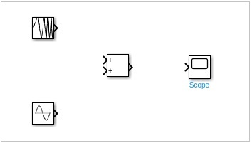
We are going to combine chirp signal and sine wave blocks by using add block from Mathoperation and see the final display.

Let us pick the block we want. Select chirp signal and sine wave from sources library, add block from math operations, scope block from sinks library.

Join the lines to each block.

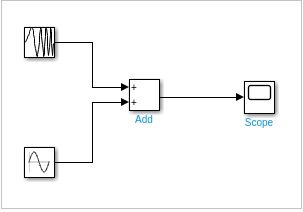
Double click chirp signal and change the initial frequency from 0.1 to 0.05 and click on Ok button.

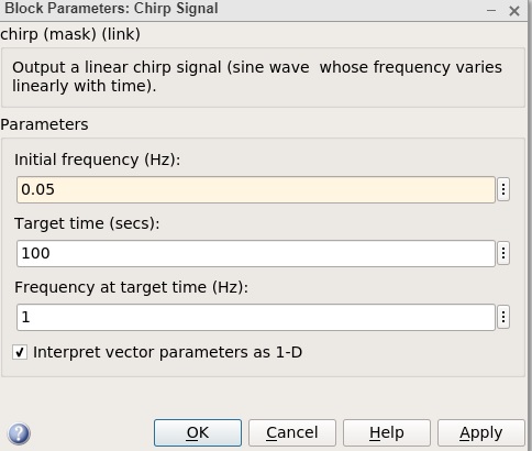
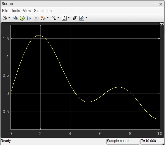
The other blocks are kept as the default values. Now, click on run to see the output in scope as shown below.

Build Model & Apply If-else Logic

In this chapter, we will create a model and apply if-else logic to it. Let us first collect blocks to create our model.

Now, open MATLAB Simulink (blank model) and the Simulink library browser as shown below −

Click on the Blank Model and open Simulink library browser as shown below −

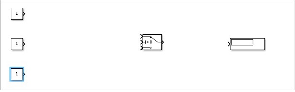
The blocks we require to build the model with if-else logic is as follows −

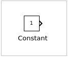
Constant block from Commonly used blocks

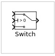
Switch block from Signal Routing

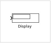
Display block from Sinks

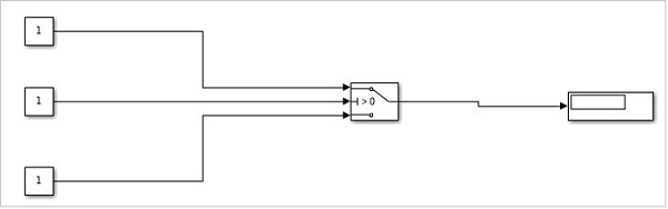
Let us now get all the blocks together to create a model as shown below −

Let us now connect the lines with each block. So you can see that the constant block has one output and the switch has three inputs and one output. We are going to connect them to the display block.

After connecting the lines, the model is as shown below −

Now, double click the switch block and add a threshold.

The threshold value will be compared with the block in the center. Based on the constant value of the middle block, the first block value will be displayed or the last constant block value will be displayed.

Let us add a threshold value to the switch as shown below −

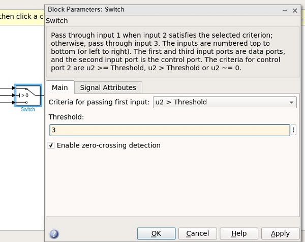
The threshold value given is 3. Click on OK to update the threshold. Now the threshold value is seen inside the switch block as shown below −

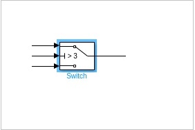
The middle constant block will be compared with the switch threshold and accordingly the display will be decided.

Let us now update the middle constant block with some value as shown below −

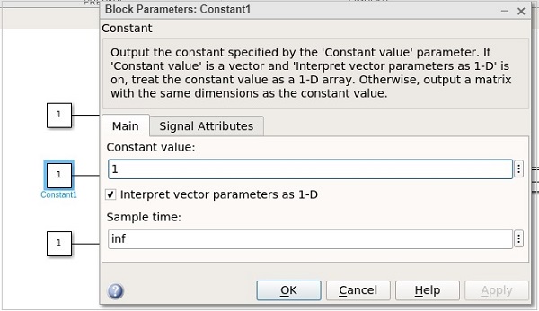
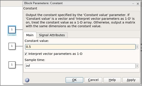
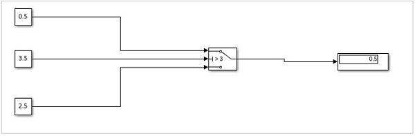
The value of the constant block is 1. Let us now change the first constant block and give it a value as 0.5 as shown below −

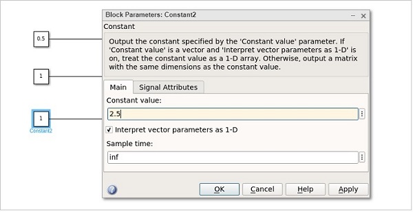
Let us now change the last constant with value as 2.5 as shown below −

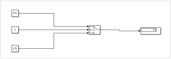
Hence, the first constant value is 0.5, the middle constant value is 1 and the last one is 2.5. The middle constant value 1 will be compared to switch threshold value i.e. 3 as (1 >3). It will print the value as 2.5 the last constant value.

Click on the run button to get the output in the display block as shown below −

Let us now change the middle constant to a higher value than the threshold of switch and see the output −

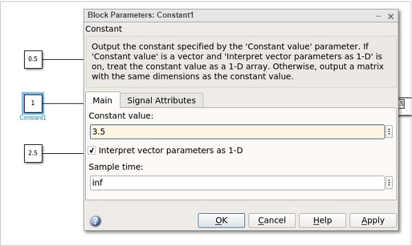
The value is changed from 1 to 3.5. Click on OK and run the model to see the output in the display −

Now, since the value of the middle constant is greater, the value from the first constant is printed in display. If it is less, then the value from the last constant will be printed.

MATLAB Simulink - Logic Gates Model

In this chapter, let us understand how to build a model that demonstrates the logic gates.

For example, gates like OR, AND, XOR etc.

Open the Simulink and open a blank model as shown below −

Click on blank model and select the Simulink library as shown below −

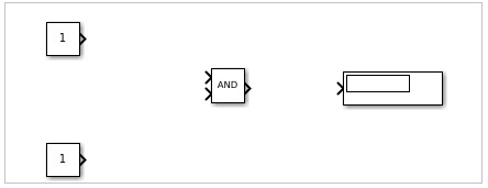
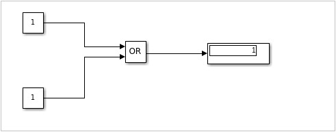
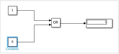
Let us select the block that we want to build a OR gate. We need two constant blocks to act as inputs, a logic operator block and a display block.

The constant and logic operator block will get from commonly used blocks library. Select the blocks and drag in your model or just type the name of the block in your model and select the block as shown below −

Select the constant block, we need two constant block, a logical operator and a constant.

The blocks will look as shown below −

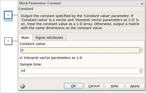
Right click on the logic operator block and it will display the block parameters as shown below −

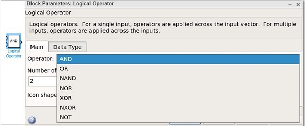
With logical operator you can use AND, OR, NAND, NOR, XOR, NXOR and NOT gates. Right now we are going to select the OR gate.

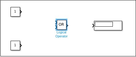
Now connect the lines and the model will be as shown below −

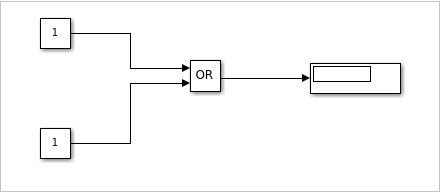
For an OR gate if the inputs are 1,1 the output will be 1. If the inputs are 0,0 the output will be 0. Right now, the constant has values 1,1. Let us run the model to see the output as shown below −

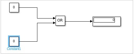
We can see in the display block the output shown is 1. Let us now change the constant value to 0. Right click on constant block and change the value as shown below −

After changing the values of constant to 0, the output will become 0 when you run the model. The output is as shown below −

Let us now change the constant values to 0,1 and see the output −

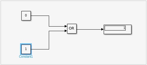
With values as 1,0, the display will be as follows −

Similarly, you can design the AND and other gates.

MATLAB Simulink - Sine Wave

In this chapter we will integrate and differentiate sine wave by using the derivative and integrator blocks.

Open blank model and Simulink library as shown below −

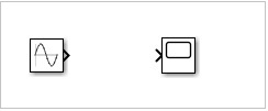
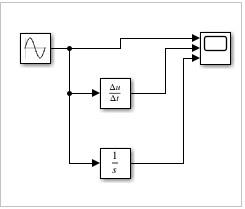
Let us pick the sine wave from sources library and scope block from sinks library.

We would like to add the derivative and integrator block from continuous library as shown below −

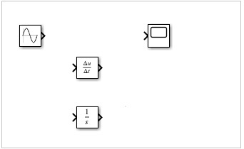
We would need 3 input ports for scope block as the sine wave, derivative and integrator block will be connected to it.

Right click on the scope block and change the inputs from 1 to 3 as shown below −

Connect the lines as shown below −

Now, run the model to see the display.

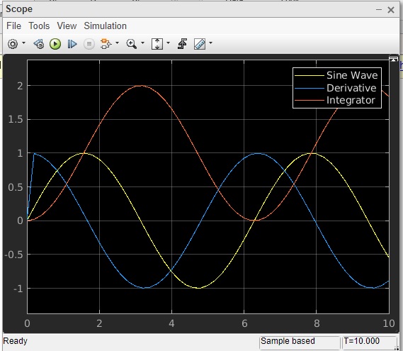
So, we have three signals sine wave, derivative and integrator.

MATLAB Simulink - Function

In this chapter we will understand how to make use of MATLAB function in Simulink.

Open Simulink and click on blank model.

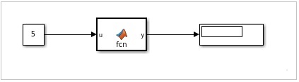
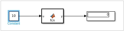
We need a constant block, a MATLAB function block and a display block for the output.

Here is the model created −

The MATLAB function is available inside the user defined functions library.

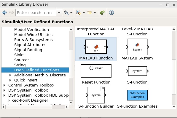
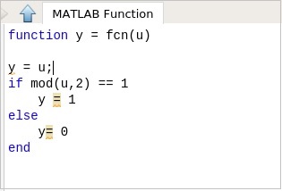
Now, click on MATLAB function and drag it inside your model canvas. Double click on the MATLAB function block and write a function of your choice.

We will try to display 1 if the number given is odd and 0 if it is even. You can also save the function to be used later with another one.

Once the function is done click on the upward arrow close to the MATLAB function and it will take you back to the model you created earlier.

Now, let us test the model by using the constant value as 5.

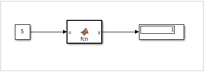
We can see the display as 1, which indicates that the value 5 is an odd number.

Let us now change the constant value to 10 as shown below and run the simulation: The output is 0 indicating it is even number.

MATLAB Simulink - Create Subsystem

Subsystems are useful when your model gets big and complex. You can change a part of the model into a subsystem that helps to keep the flow very clean and understandable.

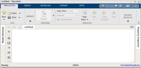
In this chapter, let us learn how to create a simple subsystem in Simulink. First, create a blank model, as shown below −

Now, we will create a simple model that adds two numbers and later converts a part of the model into a subsystem.

We have created a simple model that has two inputs. These inputs will add up and show the result inside the display.

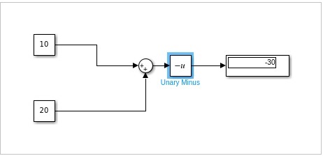
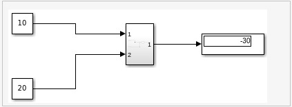
We will change the value of the constant as 10 and 20. The result 10+20 = 30 should be seen inside the display block.

Let us add one more block named Unary minus that will change the output from 30 to -30 as shown below −

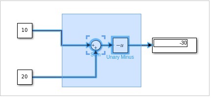
Now, let us select the portion i.e. the sum and the Unary minus block to create a subsystem as shown below −

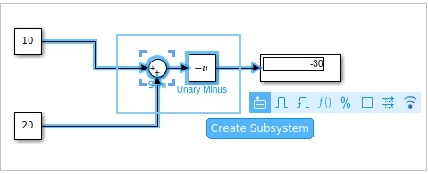
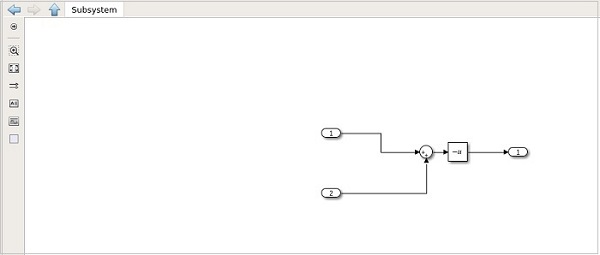
Click on Create Subsystem. Once done, the sum block and the Unary minus block will be converted into a subsystem as shown below −

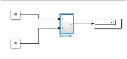
Now when you run the simulation, it will display the same result as earlier

Double click on the subsystem to see the original block as shown below −

Click on the upward arrow close to the subsystem to get back to the model.

MATLAB Simulink - For Loop

In this chapter, let us understand the working of for-iterator block. First, create a blank model as shown below −

In this model, we are going to make use of for iterator that will give us the sum of 1..N.

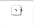
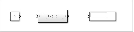
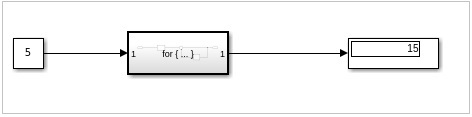
You can use the value of n as per your choice. This value will take the constant block and update it with value 5 as shown below −

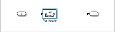
Let us add the for-iterator block as shown below −

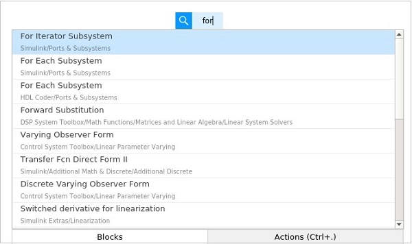
Select the for Iterator subsystem block and add to your model. Next, we need display block as shown below −

Connect the blocks as shown below −

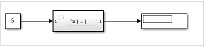
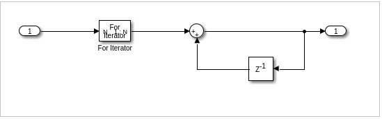
The for iterator block is a subsystem. Select the block and click enter. It will take you to new model area, where the for block has to be defined.

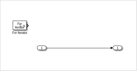
Right click on the for iterator and select the block parameters, as shown below −

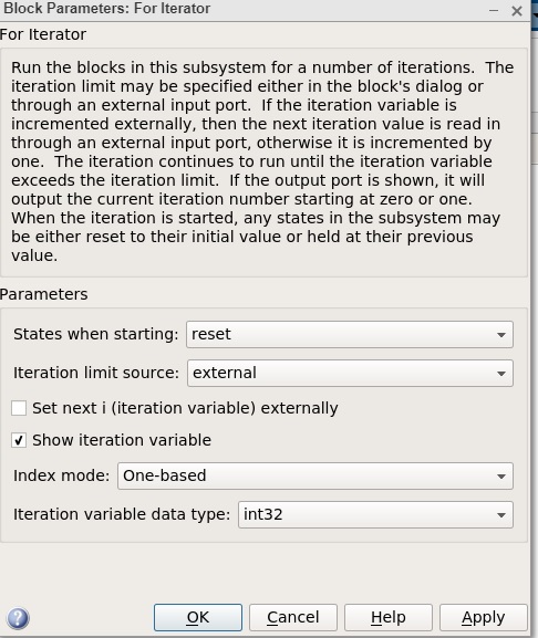
Change the States when starting as reset and Iteration limit source as external. Click on Ok to update the changes.

Now, you will get an input block to your for loop, as given below −

We need a sum block and a delay block as shown below −

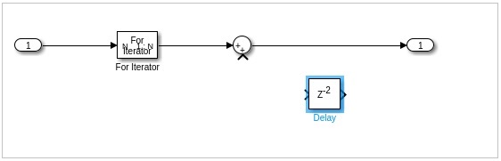
The delay block has to be flipped so that it can be added to the output. We need to give the output back to the sum block so that it can be added with the current iteration.

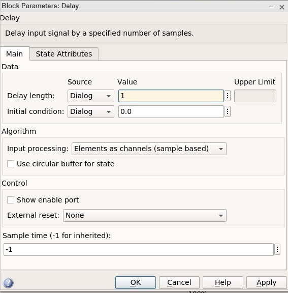
Right click on delay block and change the delay length from 2 to 1 as shown below. Click on OK to update the changes.

The final for-loop subsystem block will look as follows −

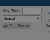
Now before you run the simulation, change the stop time to 1. We do this because we want the simulation to run only once.

Click on Run now to see the result in display block as shown below

The input value is 5, so the for-loop will go from 1 to 5. Hence, the values 1+2+3+4+5 = 15 is shown in the display.

MATLAB Simulink - Export Data

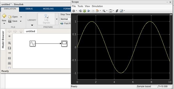
In this chapter, we will learn how to use Simulink output results inside MATLAB. Let us try a simple model of sine wave as shown below −

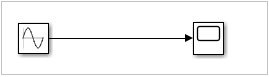
When we run the model, the scope displays the sine wave as shown below −

Now to get the data of the sine wave, go to the configuration properties and select logging tab.

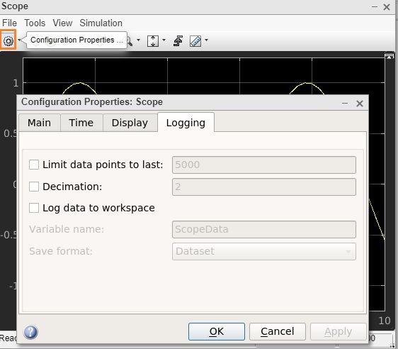
Select the log data to workspace checkbox, as shown below −

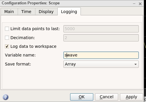
Set the variable name of your choice. Here, we have given the name as swave and the save format as Array. Click on OK button and run the simulation again.

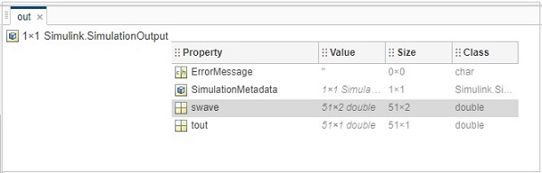
You should see the output in the workspace

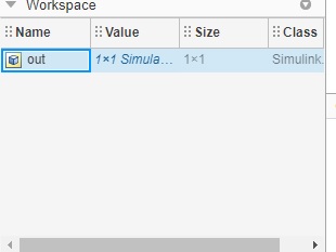
Double click and it will show you the details of the swave variable which we saved earlier.

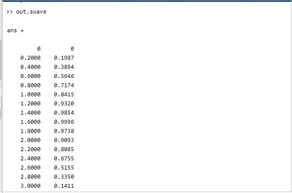
Inside command prompt type out .swave and it will give you the output as shown below −

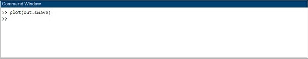
You can plot the sine wave using plot command as shown below −

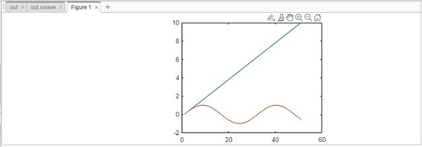
The graph is shown as follows −

MATLAB Simulink - MATLAB Script

In this chapter, we will use MATLAB script to create a model. We do have a direct and easy method to create a model by just picking the blocks we need. But, writing the code to create a model can sometimes help you to automate a task as your projects get complex.

So, let us learn how to create models by using the Application Programming Interfaces (APIs) as discussed below.

We will create a very simple sine wave model. For that we need sine wave and scope blocks.

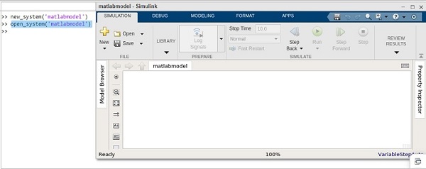
Inside the MATLAB command window, we can use API to create the model and blocks. To create a new model, the API is as follows −

new_system('matlabmodel')

Here, matlabmodel is the name of the model. You can open the model by using open_system() with the name of the model as parameter to the function.

The command is as shown below −

open_system('matlabmodel')

When you click enter, the model is opened as shown below −

Now, let us add sine wave block to it. The command is to add_block(source, dest).

You will get the source of the block from Simulink library browser.

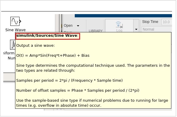
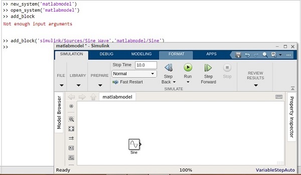
The highlighted code is the source of sine wave. Let us add that in the add_block as shown below −

add_block('simulink/Sources/Sine Wave','matlabmodel/Sine')

The following screen will appear on your computer −

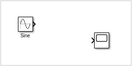
Let us now add the scope block, as mentioned below −

add_block('simulink/Sinks/Scope','matlabmodel/Scope', ‘Position’ , [200 315 135 50])

The model shows the scope block as shown below −

You can make use of position inside the add_block to position the block properly.

For example,

add_block(‘simulink/Sinks/Scope’, ‘matlabmodel/Scope’, ‘Position’ , [200 315 135 50]

Now, let us connect the line between the sine wave and scope by using the command as shown below −

add_line('matlabmodel', 'Sine/1', 'Scope/1');

For add_line, you have to pass the name of your model, followed by the block name and the input port of the blocks.

So now, we want to connect the first output port of sine wave with the first input port of scope.

Let us now run the simulation by using the command below −

result = sim('matlabmodel');

Now to view the simulation result, run one more command as shown below −

open_system('matlabmodel/Scope');

You will get the output inside the scope as follows −

Solving Mathematical Equation

In this chapter, we will solve a simple mathematical equation by using Simulink.

The equation is given below −

y(t) = 2Sin(t) + 5Sin(2t) - 10

Let us create a model for the above equation. Open a blank model as shown below −

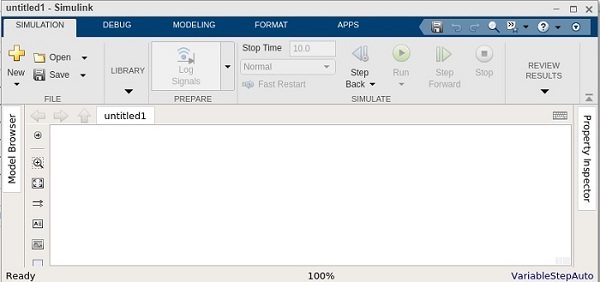
Following are the steps to solve the equation −

Get a Sine wave block. Right click and select block parameters. Select sign type as time based. Change the amplitude to 2 and frequency to 1. That will be 2Sin(t).
Get another sine wave block. Now, set the amplitude to 5 and frequency to 2 to display 5Sin(2t). Select sign type as time based.
Now get an add block and add both sine waves.
Get a constant. Right click and select block parameters. Change the value from 1 to 10.
Get a subtract block where one input will come from step 3 and another from constant i.e. step 4.
Get a scope block and connect the input from step 6 to it.

This is how the final Simulink model looks like for the equation −

y(t) = 2Sin(t) + 5Sin(2t) - 10

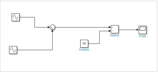
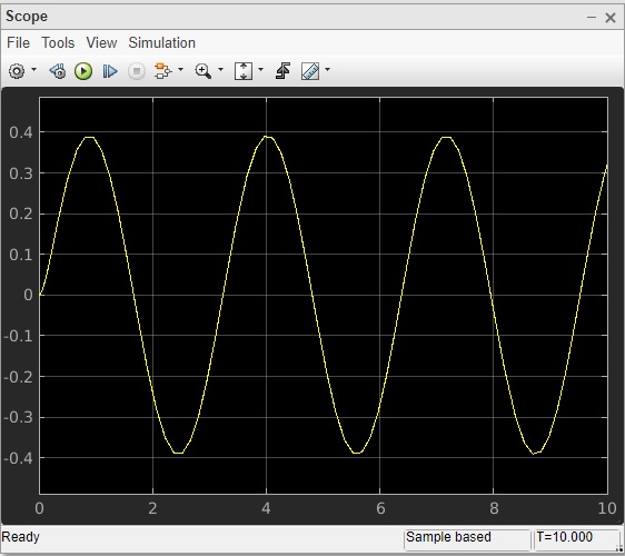
Click on the run button to compile. Right Click on scope block to see the signal plotted.

First Order Differential Equation

Here, we will learn how to solve the first order differential equation in Simulink.

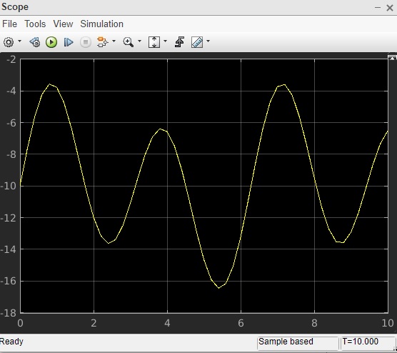
The first order differential equation that we are trying to solve using Simulink is as follows −

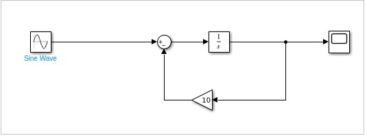
dy/dt = 4sin2t - 10y

The equation can be solved by integrating dy/dt to the following −

y(t)=∫(4sin2t - 10y(t))dt

Following are the steps to build a model for above equation.

Pick up sine wave from sources library and change the amplitude to 4 and frequency to 2. This will give us 4sin2t.
The integrator block will be used to show dy/dt that will give output y(t).
The gain block will represent 10y.
The input of step 1 and 3 will be given to step2.
We need scope block to see the output y(t). The step 4 will be connected to the scope block.

Let us see the above steps in model as shown below −

Run the block to see the following output −