- SciPy - Home
- SciPy - Introduction
- SciPy - Environment Setup
- SciPy - Basic Functionality
- SciPy - Relationship with NumPy
- SciPy Clusters
- SciPy - Clusters
- SciPy - Hierarchical Clustering
- SciPy - K-means Clustering
- SciPy - Distance Metrics
- SciPy Constants
- SciPy - Constants
- SciPy - Mathematical Constants
- SciPy - Physical Constants
- SciPy - Unit Conversion
- SciPy - Astronomical Constants
- SciPy - Fourier Transforms
- SciPy - FFTpack
- SciPy - Discrete Fourier Transform (DFT)
- SciPy - Fast Fourier Transform (FFT)
- SciPy Integration Equations
- SciPy - Integrate Module
- SciPy - Single Integration
- SciPy - Double Integration
- SciPy - Triple Integration
- SciPy - Multiple Integration
- SciPy Differential Equations
- SciPy - Differential Equations
- SciPy - Integration of Stochastic Differential Equations
- SciPy - Integration of Ordinary Differential Equations
- SciPy - Discontinuous Functions
- SciPy - Oscillatory Functions
- SciPy - Partial Differential Equations
- SciPy Interpolation
- SciPy - Interpolate
- SciPy - Linear 1-D Interpolation
- SciPy - Polynomial 1-D Interpolation
- SciPy - Spline 1-D Interpolation
- SciPy - Grid Data Multi-Dimensional Interpolation
- SciPy - RBF Multi-Dimensional Interpolation
- SciPy - Polynomial & Spline Interpolation
- SciPy Curve Fitting
- SciPy - Curve Fitting
- SciPy - Linear Curve Fitting
- SciPy - Non-Linear Curve Fitting
- SciPy - Input & Output
- SciPy - Input & Output
- SciPy - Reading & Writing Files
- SciPy - Working with Different File Formats
- SciPy - Efficient Data Storage with HDF5
- SciPy - Data Serialization
- SciPy Linear Algebra
- SciPy - Linalg
- SciPy - Matrix Creation & Basic Operations
- SciPy - Matrix LU Decomposition
- SciPy - Matrix QU Decomposition
- SciPy - Singular Value Decomposition
- SciPy - Cholesky Decomposition
- SciPy - Solving Linear Systems
- SciPy - Eigenvalues & Eigenvectors
- SciPy Image Processing
- SciPy - Ndimage
- SciPy - Reading & Writing Images
- SciPy - Image Transformation
- SciPy - Filtering & Edge Detection
- SciPy - Top Hat Filters
- SciPy - Morphological Filters
- SciPy - Low Pass Filters
- SciPy - High Pass Filters
- SciPy - Bilateral Filter
- SciPy - Median Filter
- SciPy - Non - Linear Filters in Image Processing
- SciPy - High Boost Filter
- SciPy - Laplacian Filter
- SciPy - Morphological Operations
- SciPy - Image Segmentation
- SciPy - Thresholding in Image Segmentation
- SciPy - Region-Based Segmentation
- SciPy - Connected Component Labeling
- SciPy Optimize
- SciPy - Optimize
- SciPy - Special Matrices & Functions
- SciPy - Unconstrained Optimization
- SciPy - Constrained Optimization
- SciPy - Matrix Norms
- SciPy - Sparse Matrix
- SciPy - Frobenius Norm
- SciPy - Spectral Norm
- SciPy Condition Numbers
- SciPy - Condition Numbers
- SciPy - Linear Least Squares
- SciPy - Non-Linear Least Squares
- SciPy - Finding Roots of Scalar Functions
- SciPy - Finding Roots of Multivariate Functions
- SciPy - Signal Processing
- SciPy - Signal Filtering & Smoothing
- SciPy - Short-Time Fourier Transform
- SciPy - Wavelet Transform
- SciPy - Continuous Wavelet Transform
- SciPy - Discrete Wavelet Transform
- SciPy - Wavelet Packet Transform
- SciPy - Multi-Resolution Analysis
- SciPy - Stationary Wavelet Transform
- SciPy - Statistical Functions
- SciPy - Stats
- SciPy - Descriptive Statistics
- SciPy - Continuous Probability Distributions
- SciPy - Discrete Probability Distributions
- SciPy - Statistical Tests & Inference
- SciPy - Generating Random Samples
- SciPy - Kaplan-Meier Estimator Survival Analysis
- SciPy - Cox Proportional Hazards Model Survival Analysis
- SciPy Spatial Data
- SciPy - Spatial
- SciPy - Special Functions
- SciPy - Special Package
- SciPy Advanced Topics
- SciPy - CSGraph
- SciPy - ODR
- SciPy Useful Resources
- SciPy - Reference
- SciPy - Quick Guide
- SciPy - Cheatsheet
- SciPy - Useful Resources
- SciPy - Discussion
SciPy - Basic Functionality
SciPy is an open-source Python library that is widely used in the scientific community for various tasks involving numerical computation. This library is built on top of NumPy.
SciPy extends its capabilities by providing additional functionality that is essential for scientific and engineering applications. This includes algorithms and functions for optimization, integration, interpolation, eigenvalue problems and solving differential equations.
Here is the overview of the basic functionalities of SciPy library −
Numerical Integration
Numerical integration refers to techniques for calculating the integral of a function when an analytical solution is difficult or impossible to obtain. SciPy provides several methods for numerical integration as discussed below −
- Quad Integration: This is used to compute the integral of a function over a specified interval. In SciPy using scipy.integrate.quad() we can perform adaptive quadrature to compute definite integrals. It returns both the integral result and an estimate of the error.
- Simpsons Rule: This is a numerical method for estimating the definite integral of a function. It is particularly effective for integrating smooth functions and is based on approximating the function by a quadratic polynomial.
This can be implemented by scipy.integrate.simps this method uses polynomial interpolation to provide a more accurate estimate than simple trapezoidal rules.
Example
Below is the example of computing the integral f(x) = e-x2, which is the area under the curve of the Gaussian function and it converges to a known value by using the quad() function of the scipy.integrate module.
from scipy import integrate
import numpy as np

# Function to integrate
def f(x):
   return np.exp(-x**2)

# Compute the integral from 0 to infinity
result, error = integrate.quad(f, 0, np.inf)
print(f"Integral result: {result}, Error estimate: {error}")
Following is the output of the quad() function −
Integral result: 0.8862269254527579, Error estimate: 7.101318378329813e-09
Optimization
Optimization involves finding the best solution i.e. maximum or minimum of a given function. SciPy offers several optimization algorithms through the scipy.optimize(). Following are the methods that optimization can be done −
- Minimization: Use functions like minimize to find the minimum of a scalar function of one or more variables. It supports various methods such as Nelder-Mead, BFGS and Powell etc.
- Root Finding: The fsolve() function helps find the roots of a system of equations.
Example
The following example shows how to use the minimize() function of the scipy.optimize module to find the minimum of a simple quadratic function −
from scipy import optimize

# Define a function to minimize
def objective_function(x):
   return (x - 2)**2 + 1

# Find the minimum of the function
result = optimize.minimize(objective_function, x0=0)
print(f"Minimum value: {result.fun} at x = {result.x}")
Following is the output of the minimize() function −
Minimum value: 1.0000000000000007 at x = [1.99999997]
Interpolation
Interpolation is a technique to estimate unknown values that fall between known data points. SciPys scipy.interpolate module provides various methods for interpolation −
- Linear and Cubic Interpolation − Use interp1d for one-dimensional interpolation which can be linear, quadratic or cubic.
- Barycentric Interpolation − This provides high-order polynomial interpolation and is more numerically stable.
Example
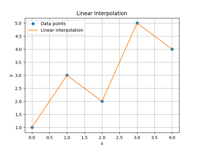
Here is the example which shows how to perform linear interpolation using SciPy and visualize the results with Matplotlib −
from scipy import interpolate
import matplotlib.pyplot as plt
import numpy as np

# Sample data
x = np.array([0, 1, 2, 3, 4])  # Original x values
y = np.array([1, 3, 2, 5, 4])  # Corresponding y values

# Create a linear interpolation function
linear_interp = interpolate.interp1d(x, y)

# New x values for interpolation
x_new = np.linspace(0, 4, 100)  # 100 points between 0 and 4
y_new = linear_interp(x_new)  # Interpolated y values

# Plot the original data and the interpolation
plt.plot(x, y, 'o', label='Data points')  # Original data points as circles
plt.plot(x_new, y_new, '-', label='Linear interpolation')  # Interpolated line
plt.legend()  # Show legend
plt.xlabel('x')
plt.ylabel('y')
plt.title('Linear Interpolation')
plt.grid()  # Add a grid
plt.show()  # Display the plot
Following is the output of the Linear interpolation −
Eigenvalue Problems
Eigenvalue problems are a fundamental concept in linear algebra, arising in various fields such as physics, engineering, and data science. They involve finding eigenvalues and eigenvectors of a matrix. An eigenvalue and its corresponding eigenvector of a square matrix satisfy the equation as defined below −
A v = λ v
Example
Below is the example which shows how to compute the eigenvalues and eigenvectors of a given matrix using the eig() function of the scipy.linalg module.
from scipy.linalg import eig
import numpy as np
# Define a matrix
A = np.array([[1, 2], [2, 1]])

# Compute eigenvalues and eigenvectors
eigenvalues, eigenvectors = eig(A)
print(f"Eigenvalues: {eigenvalues}")
print(f"Eigenvectors:\n{eigenvectors}")
Here is the output of the eigenvalues and eigenvectors of a given matrix −
Eigenvalues: [ 3.+0.j -1.+0.j]
Eigenvectors:
[[ 0.70710678 -0.70710678]
 [ 0.70710678  0.70710678]]
Algebraic Equations
SciPy provides tools for solving linear algebraic equations. The scipy.linalg module includes functions for matrix operations, solving linear systems and computing determinants.
Example
This is the example which shows how to use the solve() function of the scipy.linalg module on linear equations −
import numpy as np
from scipy.linalg import solve

# Define a coefficient matrix A and a right-hand side vector b
A = np.array([[3, 2], [1, 2]])
b = np.array([5, 5])

# Solve the linear system
x = solve(A, b)
print(f"Solution of the linear system: {x}")
Following is the output of the above program −
Solution of the linear system: [0. 2.5]
Statistical Functions
SciPy also includes the scipy.stats module which contains a large collection of statistical distributions and functions for statistical testing.
- Probability Distributions: SciPy supports many continuous and discrete distributions such as normal, binomial, Poisson etc.
- Statistical Tests: There are functions for performing statistical tests such as t-tests and chi-square tests.
Example
This example shows how to perform a Shapiro-Wilk test for normality using the scipy.stats module in Python. This statistical test checks whether a given dataset follows a normal distribution −
from scipy import stats
import numpy as np
# Generate random data
data = np.random.normal(0, 1, 1000)

# Perform a Shapiro-Wilk test for normality
statistic, p_value = stats.shapiro(data)
print(f"Shapiro-Wilk test statistic: {statistic}, p-value: {p_value}")
Following is the output of the above program −
Shapiro-Wilk test statistic: 0.9984066795076805, p-value: 0.49518026390115066