- Python Deep Learning - Home
- Python Deep Learning - Introduction
- Python Deep Learning - Environment
- Python Deep Learning - Basic Machine Learning
- Python Deep Learning - Artificial Neural Networks
- Python Deep Learning - Deep Neural Networks
- Python Deep Learning - Fundamentals
- Python Deep Learning - Training Neural Network
- Python Deep Learning - Computational Graphs
- Python Deep Learning - Applications
- Python Deep Learning - Libraries and Frameworks
- Python Deep Learning - Implementations
Python Deep Learning Resources
Python Deep Learning - Deep Learning Implementations
In this implementation of Deep learning, our objective is to predict the customer attrition or churning data for a certain bank - which customers are likely to leave this bank service. The Dataset used is relatively small and contains 10000 rows with 14 columns. We are using Anaconda distribution, and frameworks like Theano, TensorFlow and Keras. Keras is built on top of Tensorflow and Theano which function as its backends.
# Artificial Neural Network
# Installing Theano
pip3 install --upgrade theano

# Installing Tensorflow
pip3 install upgrade tensorflow

# Installing Keras
pip3 install --upgrade keras
Step 1: Data preprocessing
In[]:

# Importing the libraries
   import numpy as np
   import matplotlib.pyplot as plt
   import pandas as pd

# Importing the database
   dataset = pd.read_csv('Churn_Modelling.csv')
Step 2
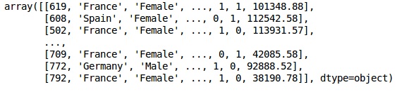
We create matrices of the features of dataset and the target variable, which is column 14, labeled as Exited.
The initial look of data is as shown below −
In[]:
X = dataset.iloc[:, 3:13].values
Y = dataset.iloc[:, 13].values
X
Output
Step 3
Y
Output
array([1, 0, 1, ..., 1, 1, 0], dtype = int64)
Step 4
We make the analysis simpler by encoding string variables. We are using the ScikitLearn function LabelEncoder to automatically encode the different labels in the columns with values between 0 to n_classes-1.
from sklearn.preprocessing import LabelEncoder, OneHotEncoder
labelencoder_X_1 = LabelEncoder()
X[:,1] = labelencoder_X_1.fit_transform(X[:,1])
labelencoder_X_2 = LabelEncoder()
X[:, 2] = labelencoder_X_2.fit_transform(X[:, 2])
X
Output
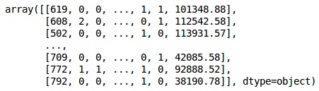
In the above output,country names are replaced by 0, 1 and 2; while male and female are replaced by 0 and 1.
Step 5
Labelling Encoded Data
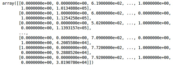
We use the same ScikitLearn library and another function called the OneHotEncoder to just pass the column number creating a dummy variable.
onehotencoder = OneHotEncoder(categorical features = [1])
X = onehotencoder.fit_transform(X).toarray()
X = X[:, 1:]
X
Now, the first 2 columns represent the country and the 4th column represents the gender.
Output
We always divide our data into training and testing part; we train our model on training data and then we check the accuracy of a model on testing data which helps in evaluating the efficiency of model.
Step 6
We are using ScikitLearns train_test_split function to split our data into training set and test set. We keep the train- to- test split ratio as 80:20.
#Splitting the dataset into the Training set and the Test Set
from sklearn.model_selection import train_test_split
X_train, X_test, y_train, y_test = train_test_split(X, y, test_size = 0.2)
Some variables have values in thousands while some have values in tens or ones. We scale the data so that they are more representative.
Step 7
In this code, we are fitting and transforming the training data using the StandardScaler function. We standardize our scaling so that we use the same fitted method to transform/scale test data.
# Feature Scaling
fromsklearn.preprocessing import StandardScaler
sc = StandardScaler()
X_train = sc.fit_transform(X_train)
X_test = sc.transform(X_test)
Output
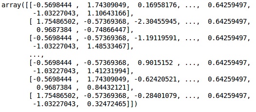
The data is now scaled properly. Finally, we are done with our data pre-processing. Now,we will start with our model.
Step 8
We import the required Modules here. We need the Sequential module for initializing the neural network and the dense module to add the hidden layers.
# Importing the Keras libraries and packages
import keras
from keras.models import Sequential
from keras.layers import Dense
Step 9
We will name the model as Classifier as our aim is to classify customer churn. Then we use the Sequential module for initialization.
#Initializing Neural Network
classifier = Sequential()
Step 10
We add the hidden layers one by one using the dense function. In the code below, we will see many arguments.
Our first parameter is output_dim. It is the number of nodes we add to this layer. init is the initialization of the Stochastic Gradient Decent. In a Neural Network we assign weights to each node. At initialization, weights should be near to zero and we randomly initialize weights using the uniform function. The input_dim parameter is needed only for first layer, as the model does not know the number of our input variables. Here the total number of input variables is 11. In the second layer, the model automatically knows the number of input variables from the first hidden layer.
Execute the following line of code to addthe input layer and the first hidden layer −
classifier.add(Dense(units = 6, kernel_initializer = 'uniform',
activation = 'relu', input_dim = 11))
Execute the following line of code to add the second hidden layer −
classifier.add(Dense(units = 6, kernel_initializer = 'uniform',
activation = 'relu'))
Execute the following line of code to add the output layer −
classifier.add(Dense(units = 1, kernel_initializer = 'uniform',
activation = 'sigmoid'))
Step 11
Compiling the ANN
We have added multiple layers to our classifier until now. We will now compile them using the compile method. Arguments added in final compilation control complete the neural network.So,we need to be careful in this step.
Here is a brief explanation of the arguments.
First argument is Optimizer.This is an algorithm used to find the optimal set of weights. This algorithm is called the Stochastic Gradient Descent (SGD). Here we are using one among several types, called the Adam optimizer. The SGD depends on loss, so our second parameter is loss. If our dependent variable is binary, we use logarithmic loss function called binary_crossentropy, and if our dependent variable has more than two categories in output, then we use categorical_crossentropy. We want to improve performance of our neural network based on accuracy, so we add metrics as accuracy.
# Compiling Neural Network
classifier.compile(optimizer = 'adam', loss = 'binary_crossentropy', metrics = ['accuracy'])
Step 12
A number of codes need to be executed in this step.
Fitting the ANN to the Training Set
We now train our model on the training data. We use the fit method to fit our model. We also optimize the weights to improve model efficiency. For this, we have to update the weights. Batch size is the number of observations after which we update the weights. Epoch is the total number of iterations. The values of batch size and epoch are chosen by the trial and error method.
classifier.fit(X_train, y_train, batch_size = 10, epochs = 50)
Making predictions and evaluating the model
# Predicting the Test set results
y_pred = classifier.predict(X_test)
y_pred = (y_pred > 0.5)
Predicting a single new observation
# Predicting a single new observation
"""Our goal is to predict if the customer with the following data will leave the bank:
Geography: Spain
Credit Score: 500
Gender: Female
Age: 40
Tenure: 3
Balance: 50000
Number of Products: 2
Has Credit Card: Yes
Is Active Member: Yes
Step 13
Predicting the test set result
The prediction result will give you probability of the customer leaving the company. We will convert that probability into binary 0 and 1.
# Predicting the Test set results
y_pred = classifier.predict(X_test)
y_pred = (y_pred > 0.5)
new_prediction = classifier.predict(sc.transform
(np.array([[0.0, 0, 500, 1, 40, 3, 50000, 2, 1, 1, 40000]])))
new_prediction = (new_prediction > 0.5)
Step 14
This is the last step where we evaluate our model performance. We already have original results and thus we can build confusion matrix to check the accuracy of our model.
Making the Confusion Matrix
from sklearn.metrics import confusion_matrix
cm = confusion_matrix(y_test, y_pred)
print (cm)
Output
loss: 0.3384 acc: 0.8605
[ [1541 54]
[230 175] ]
From the confusion matrix, the Accuracy of our model can be calculated as −
Accuracy = 1541+175/2000=0.858
We achieved 85.8% accuracy, which is good.
The Forward Propagation Algorithm
In this section, we will learn how to write code to do forward propagation (prediction) for a simple neural network −
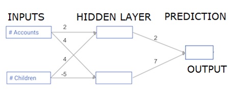
Each data point is a customer. The first input is how many accounts they have, and the second input is how many children they have. The model will predict how many transactions the user makes in the next year.
The input data is pre-loaded as input data, and the weights are in a dictionary called weights. The array of weights for the first node in the hidden layer are in weights [node_0], and for the second node in the hidden layer are in weights[node_1] respectively.
The weights feeding into the output node are available in weights.
The Rectified Linear Activation Function
An "activation function" is a function that works at each node. It transforms the node's input into some output.
The rectified linear activation function (called ReLU) is widely used in very high-performance networks. This function takes a single number as an input, returning 0 if the input is negative, and input as the output if the input is positive.
Here are some examples −
- relu(4) = 4
- relu(-2) = 0
We fill in the definition of the relu() function−
- We use the max() function to calculate the value for the output of relu().
- We apply the relu() function to node_0_input to calculate node_0_output.
- We apply the relu() function to node_1_input to calculate node_1_output.
import numpy as np
input_data = np.array([-1, 2])
weights = {
   'node_0': np.array([3, 3]),
   'node_1': np.array([1, 5]),
   'output': np.array([2, -1])
}
node_0_input = (input_data * weights['node_0']).sum()
node_0_output = np.tanh(node_0_input)
node_1_input = (input_data * weights['node_1']).sum()
node_1_output = np.tanh(node_1_input)
hidden_layer_output = np.array(node_0_output, node_1_output)
output =(hidden_layer_output * weights['output']).sum()
print(output)

def relu(input):
   '''Define your relu activation function here'''
   # Calculate the value for the output of the relu function: output
   output = max(input,0)
      # Return the value just calculated
   return(output)
# Calculate node 0 value: node_0_output
node_0_input = (input_data * weights['node_0']).sum()
node_0_output = relu(node_0_input)

# Calculate node 1 value: node_1_output
node_1_input = (input_data * weights['node_1']).sum()
node_1_output = relu(node_1_input)

# Put node values into array: hidden_layer_outputs
hidden_layer_outputs = np.array([node_0_output, node_1_output])

# Calculate model output (do not apply relu)
odel_output = (hidden_layer_outputs * weights['output']).sum()
print(model_output)# Print model output
Output
0.9950547536867305
-3
Applying the network to many Observations/rows of data
In this section, we will learn how to define a function called predict_with_network(). This function will generate predictions for multiple data observations, taken from network above taken as input_data. The weights given in above network are being used. The relu() function definition is also being used.
Let us define a function called predict_with_network() that accepts two arguments - input_data_row and weights - and returns a prediction from the network as the output.
We calculate the input and output values for each node, storing them as: node_0_input, node_0_output, node_1_input, and node_1_output.
To calculate the input value of a node, we multiply the relevant arrays together and compute their sum.
To calculate the output value of a node, we apply the relu()function to the input value of the node. We use a for loop to iterate over input_data −
We also use our predict_with_network() to generate predictions for each row of the input_data - input_data_row. We also append each prediction to results.
# Define predict_with_network()
def predict_with_network(input_data_row, weights):
   # Calculate node 0 value
   node_0_input = (input_data_row * weights['node_0']).sum()
   node_0_output = relu(node_0_input)

   # Calculate node 1 value
   node_1_input = (input_data_row * weights['node_1']).sum()
   node_1_output = relu(node_1_input)

   # Put node values into array: hidden_layer_outputs
   hidden_layer_outputs = np.array([node_0_output, node_1_output])

   # Calculate model output
   input_to_final_layer = (hidden_layer_outputs*weights['output']).sum()
   model_output = relu(input_to_final_layer)
# Return model output
   return(model_output)

# Create empty list to store prediction results
results = []
for input_data_row in input_data:
   # Append prediction to results
   results.append(predict_with_network(input_data_row, weights))
print(results)# Print results
Output
[0, 12]
Here we have used the relu function where relu(26) = 26 and relu(-13)=0 and so on.
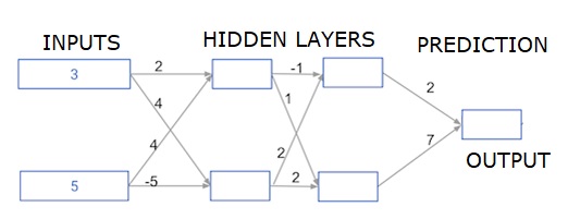
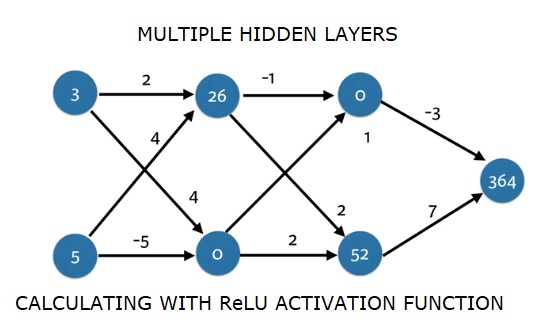
Deep multi-layer neural networks
Here we are writing code to do forward propagation for a neural network with two hidden layers. Each hidden layer has two nodes. The input data has been preloaded as input_data. The nodes in the first hidden layer are called node_0_0 and node_0_1.
Their weights are pre-loaded as weights['node_0_0'] and weights['node_0_1'] respectively.
The nodes in the second hidden layer are called node_1_0 and node_1_1. Their weights are pre-loaded as weights['node_1_0'] and weights['node_1_1'] respectively.
We then create a model output from the hidden nodes using weights pre-loaded as weights['output'].
We calculate node_0_0_input using its weights weights['node_0_0'] and the given input_data. Then apply the relu() function to get node_0_0_output.
We do the same as above for node_0_1_input to get node_0_1_output.
We calculate node_1_0_input using its weights weights['node_1_0'] and the outputs from the first hidden layer - hidden_0_outputs. We then apply the relu() function to get node_1_0_output.
We do the same as above for node_1_1_input to get node_1_1_output.
We calculate model_output using weights['output'] and the outputs from the second hidden layer hidden_1_outputs array. We do not apply the relu()function to this output.
import numpy as np
input_data = np.array([3, 5])
weights = {
   'node_0_0': np.array([2, 4]),
   'node_0_1': np.array([4, -5]),
   'node_1_0': np.array([-1, 1]),
   'node_1_1': np.array([2, 2]),
   'output': np.array([2, 7])
}
def predict_with_network(input_data):
   # Calculate node 0 in the first hidden layer
   node_0_0_input = (input_data * weights['node_0_0']).sum()
   node_0_0_output = relu(node_0_0_input)

   # Calculate node 1 in the first hidden layer
   node_0_1_input = (input_data*weights['node_0_1']).sum()
   node_0_1_output = relu(node_0_1_input)

   # Put node values into array: hidden_0_outputs
   hidden_0_outputs = np.array([node_0_0_output, node_0_1_output])

   # Calculate node 0 in the second hidden layer
   node_1_0_input = (hidden_0_outputs*weights['node_1_0']).sum()
   node_1_0_output = relu(node_1_0_input)

   # Calculate node 1 in the second hidden layer
   node_1_1_input = (hidden_0_outputs*weights['node_1_1']).sum()
   node_1_1_output = relu(node_1_1_input)

   # Put node values into array: hidden_1_outputs
   hidden_1_outputs = np.array([node_1_0_output, node_1_1_output])

   # Calculate model output: model_output
   model_output = (hidden_1_outputs*weights['output']).sum()
      # Return model_output
   return(model_output)
output = predict_with_network(input_data)
print(output)
Output
364