- Python Deep Learning - Home
- Python Deep Learning - Introduction
- Python Deep Learning - Environment
- Python Deep Learning - Basic Machine Learning
- Python Deep Learning - Artificial Neural Networks
- Python Deep Learning - Deep Neural Networks
- Python Deep Learning - Fundamentals
- Python Deep Learning - Training Neural Network
- Python Deep Learning - Computational Graphs
- Python Deep Learning - Applications
- Python Deep Learning - Libraries and Frameworks
- Python Deep Learning - Implementations
Python Deep Learning Resources
Computational Graphs
Backpropagation is implemented in deep learning frameworks like Tensorflow, Torch, Theano, etc., by using computational graphs. More significantly, understanding back propagation on computational graphs combines several different algorithms and its variations such as backprop through time and backprop with shared weights. Once everything is converted into a computational graph, they are still the same algorithm − just back propagation on computational graphs.
What is Computational Graph
A computational graph is defined as a directed graph where the nodes correspond to mathematical operations. Computational graphs are a way of expressing and evaluating a mathematical expression.
For example, here is a simple mathematical equation −
$$p = x+y$$
We can draw a computational graph of the above equation as follows.
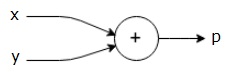
The above computational graph has an addition node (node with "+" sign) with two input variables x and y and one output q.
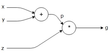
Let us take another example, slightly more complex. We have the following equation.
$$g = \left (x+y \right ) \ast z $$
The above equation is represented by the following computational graph.
Computational Graphs and Backpropagation
Computational graphs and backpropagation, both are important core concepts in deep learning for training neural networks.
Forward Pass
Forward pass is the procedure for evaluating the value of the mathematical expression represented by computational graphs. Doing forward pass means we are passing the value from variables in forward direction from the left (input) to the right where the output is.
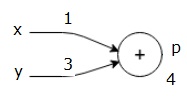
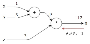
Let us consider an example by giving some value to all of the inputs. Suppose, the following values are given to all of the inputs.
$$x=1, y=3, z=3$$
By giving these values to the inputs, we can perform forward pass and get the following values for the outputs on each node.
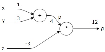
First, we use the value of x = 1 and y = 3, to get p = 4.
Then we use p = 4 and z = -3 to get g = -12. We go from left to right, forwards.
Objectives of Backward Pass
In the backward pass, our intention is to compute the gradients for each input with respect to the final output. These gradients are essential for training the neural network using gradient descent.
For example, we desire the following gradients.
Desired gradients
$$\frac{\partial x}{\partial f}, \frac{\partial y}{\partial f}, \frac{\partial z}{\partial f}$$
Backward pass (backpropagation)
We start the backward pass by finding the derivative of the final output with respect to the final output (itself!). Thus, it will result in the identity derivation and the value is equal to one.
$$\frac{\partial g}{\partial g} = 1$$
Our computational graph now looks as shown below −
Next, we will do the backward pass through the "*" operation. We will calculate the gradients at p and z. Since g = p*z, we know that −
$$\frac{\partial g}{\partial z} = p$$
$$\frac{\partial g}{\partial p} = z$$
We already know the values of z and p from the forward pass. Hence, we get −
$$\frac{\partial g}{\partial z} = p = 4$$
and
$$\frac{\partial g}{\partial p} = z = -3$$
We want to calculate the gradients at x and y −
$$\frac{\partial g}{\partial x}, \frac{\partial g}{\partial y}$$
However, we want to do this efficiently (although x and g are only two hops away in this graph, imagine them being really far from each other). To calculate these values efficiently, we will use the chain rule of differentiation. From chain rule, we have −
$$\frac{\partial g}{\partial x}=\frac{\partial g}{\partial p}\ast \frac{\partial p}{\partial x}$$
$$\frac{\partial g}{\partial y}=\frac{\partial g}{\partial p}\ast \frac{\partial p}{\partial y}$$
But we already know the dg/dp = -3, dp/dx and dp/dy are easy since p directly depends on x and y. We have −
$$p=x+y\Rightarrow \frac{\partial x}{\partial p} = 1, \frac{\partial y}{\partial p} = 1$$
Hence, we get −
$$\frac{\partial g} {\partial f} = \frac{\partial g} {\partial p}\ast \frac{\partial p} {\partial x} = \left ( -3 \right ).1 = -3$$
In addition, for the input y −
$$\frac{\partial g} {\partial y} = \frac{\partial g} {\partial p}\ast \frac{\partial p} {\partial y} = \left ( -3 \right ).1 = -3$$
The main reason for doing this backwards is that when we had to calculate the gradient at x, we only used already computed values, and dq/dx (derivative of node output with respect to the same node's input). We used local information to compute a global value.
Steps for training a neural network
Follow these steps to train a neural network −
For data point x in dataset,we do forward pass with x as input, and calculate the cost c as output.
We do backward pass starting at c, and calculate gradients for all nodes in the graph. This includes nodes that represent the neural network weights.
We then update the weights by doing W = W - learning rate * gradients.
We repeat this process until stop criteria is met.