- Managerial Economics - Home
- Managerial Economics Overview
- Business Firms & Decisions
- Economic Analysis & Optimizations
- Regression Technique
- Production & Cost Analysis
- Theory of Production
- Cost & Breakeven Analysis
- Market Structure & Pricing Theory
- Market Structure & Pricing Decisions
- Pricing Strategies
- Capital Budgeting
- Investment Under Certainty
- Investment Under Uncertainty
- Macroeconomic Aspects
- Macroeconomics Basics
- Circular Flow Model of Economy
- National Income & Measurement
- National Income Determination
- Theories of Economic Growth
- Business Cycles & Stabilization
- Inflation & ITS Control Measures
- Managerial Economics Resources
- Managerial Economics - Quick Guide
- Managerial Economics - Resources
- Managerial Economics - Discussion
Managerial Economics - Quick Guide
Managerial Economics - Overview
A close interrelationship between management and economics had led to the development of managerial economics. Economic analysis is required for various concepts such as demand, profit, cost, and competition. In this way, managerial economics is considered as economics applied to problems of choice or alternatives and allocation of scarce resources by the firms.
Managerial economics is a discipline that combines economic theory with managerial practice. It helps in covering the gap between the problems of logic and the problems of policy. The subject offers powerful tools and techniques for managerial policy making.
Managerial Economics − Definition
To quote Mansfield, Managerial economics is concerned with the application of economic concepts and economic analysis to the problems of formulating rational managerial decisions.
Spencer and Siegelman have defined the subject as the integration of economic theory with business practice for the purpose of facilitating decision making and forward planning by management.
Micro, Macro, and Managerial Economics Relationship
Microeconomics studies the actions of individual consumers and firms; managerial economics is an applied specialty of this branch. Macroeconomics deals with the performance, structure, and behavior of an economy as a whole. Managerial economics applies microeconomic theories and techniques to management decisions. It is more limited in scope as compared to microeconomics. Macroeconomists study aggregate indicators such as GDP, unemployment rates to understand the functions of the whole economy.
Microeconomics and managerial economics both encourage the use of quantitative methods to analyze economic data. Businesses have finite human and financial resources; managerial economic principles can aid management decisions in allocating these resources efficiently. Macroeconomics models and their estimates are used by the government to assist in the development of economic policy.
Nature and Scope of Managerial Economics
The most important function in managerial economics is decision-making. It involves the complete course of selecting the most suitable action from two or more alternatives. The primary function is to make the most profitable use of resources which are limited such as labor, capital, land etc. A manager is very careful while taking decisions as the future is uncertain; he ensures that the best possible plans are made in the most effective manner to achieve the desired objective which is profit maximization.
Economic theory and economic analysis are used to solve the problems of managerial economics.
Economics basically comprises of two main divisions namely Micro economics and Macro economics.
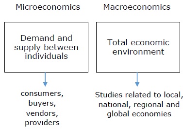
Managerial economics covers both macroeconomics as well as microeconomics, as both are equally important for decision making and business analysis.
Macroeconomics deals with the study of entire economy. It considers all the factors such as government policies, business cycles, national income, etc.
Microeconomics includes the analysis of small individual units of economy such as individual firms, individual industry, or a single individual consumer.
All the economic theories, tools, and concepts are covered under the scope of managerial economics to analyze the business environment. The scope of managerial economics is a continual process, as it is a developing science. Demand analysis and forecasting, profit management, and capital management are also considered under the scope of managerial economics.
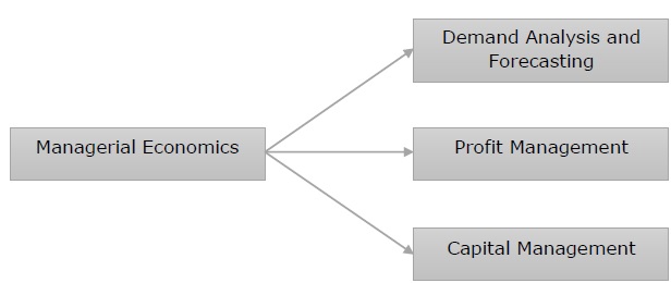
Demand Analysis and Forecasting
Demand analysis and forecasting involves huge amount of decision-making! Demand estimation is an integral part of decision making, an assessment of future sales helps in strengthening the market position and maximizing profit. In managerial economics, demand analysis and forecasting holds a very important place.
Profit Management
Success of a firm depends on its primary measure and that is profit. Firms are operated to earn long term profit which is generally the reward for risk taking. Appropriate planning and measuring profit is the most important and challenging area of managerial economics.
Capital Management
Capital management involves planning and controlling of expenses. There are many problems related to capital investments which involve considerable amount of time and labor. Cost of capital and rate of return are important factors of capital management.
Demand for Managerial Economics
The demand for this subject has increased post liberalization and globalization period primarily because of increasing use of economic logic, concepts, tools and theories in the decision making process of large multinationals.
Also, this can be attributed to increasing demand for professionally trained management personnel, who can leverage limited resources available to them and maximize returns with efficiency and effectiveness.
Role in Managerial Decision Making
Managerial economics leverages economic concepts and decision science techniques to solve managerial problems. It provides optimal solutions to managerial decision making issues.
Business Firms & Decisions
Business firms are a combination of manpower, financial, and physical resources which help in making managerial decisions. Societies can be classified into two main categories − production and consumption. Firms are the economic entities and are on the production side, whereas consumers are on the consumption side.
The performances of firms get analyzed in the framework of an economic model. The economic model of a firm is called the theory of the firm. Business decisions include many vital decisions like whether a firm should undertake research and development program, should a company launch a new product, etc.
Business decisions made by the managers are very important for the success and failure of a firm. Complexity in the business world continuously grows making the role of a manager or a decision maker of an organisation more challenging! The impact of goods production, marketing, and technological changes highly contribute to the complexity of the business environment.
Steps for Decision-Making
The steps for decision making like problem description, objective determination, discovering alternatives, forecasting consequences are described below −
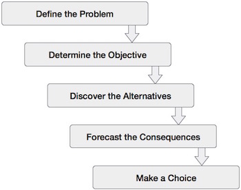
Define the Problem
What is the problem and how does it influence managerial objectives are the main questions. Decisions are usually made in the firms planning process. Managerial decisions are at times not very well defined and thus are sometimes source of a problem.
Determine the Objective
The goal of an organization or decision maker is very important. In practice, there may be many problems while setting the objectives of a firm related to profit maximization and benefit cost analysis. Are the future benefits worth the present capital? Should a firm make an investment for higher profits for over 8 to 10 years? These are the questions asked before determining the objectives of a firm.
Discover the Alternatives
For a sound decision framework, there are many questions which are needed to be answered such as − What are the alternatives? What factors are under the decision makers control? What variables constrain the choice of options? The manager needs to carefully formulate all such questions in order to weigh the attractive alternatives.
Forecast the Consequences
Forecasting or predicting the consequences of each alternative should be considered. Conditions could change by applying each alternative action so it is crucial to decide which alternative action to use when outcomes are uncertain.
Make a Choice
Once all the analysis and scrutinizing is completed, the preferred course of action is selected. This step of the process is said to occupy the lions share in analysis. In this step, the objectives and outcomes are directly quantifiable. It all depends on how the decision maker puts the problem, how he formalizes the objectives, considers the appropriate alternatives, and finds out the most preferable course of action.
Sensitivity Analysis
Sensitivity analysis helps us in determining the strong features of the optimal choice of action. It helps us to know how the optimal decision changes, if conditions related to the solution are altered. Thus, it proves that the optimal solution chosen should be based on the objective and well structured. Sensitivity analysis reflects how an optimal solution is affected, if the important factors vary or are altered.
Managerial economics is competent enough for serving the purposes in decision making. It focuses on the theory of the firm which considers profit maximization as the main objective. The theory of the firm was developed in the nineteenth century by French and English economists. Theory of the firm emphasizes on optimum utilization of resources, cost control, and profits in a single time period. Theory of the firm approach, with its focus on optimization, is relevant for small farms and producers.
Economic Analysis & Optimizations
Economic analysis is the most crucial phase in managerial economics. A manager has to collect and study the economic data of the environment in which a firm operates. He has to conduct a detailed statistical analysis in order to do research on industrial markets. The research may comprise of information regarding tax rates, products, competitors pricing strategies, etc., which may be useful for managerial decision-making.
Optimization techniques are very crucial activities in managerial decision-making process. According to the objective of the firm, the manager tries to make the most effective decision out of all the alternatives available. Though the optimal decisions differ from company to company, the objective of optimization technique is to obtain a condition under which the marginal revenue is equal to the marginal cost.
The first step in presenting optimization techniques is to examine the methods to express economic relationship. Now lets have a look at the methods of expressing economic relationship −
Equations, graphs, and tables are extensively used for expressing economic relationships.
Graphs and tables are used for simple relationships and equations are used for complex relationships.
Expressing relationships through equations is very useful in economics as it allows the usage of powerful differential technique, in order to determine the optimal solution of the problem.
Now suppose, we have total revenue equation −
TR = 100Q − 10Q2
Substituting values for quantity sold, we generate the total revenue schedule of the firm −
| 100Q − 10Q2 | TR |
|---|---|
| 100(0) − 10(0)2 | $0 |
| 100(1) − 10(1)2 | $90 |
| 100(2) − 10(2)2 | $160 |
| 100(3) − 10(3)2 | $210 |
| 100(4) − 10(4)2 | $240 |
| 100(5) − 10(5)2 | $250 |
| 100(6) − 10(6)2 | $240 |
Relationship between total, marginal, average concepts, and measures is really crucial in managerial economics. Total cost comprises of total fixed cost plus total variable cost or average cost multiply by total number of units produced
TC = TFC + TVC or TC = AC.Q
Marginal cost is the change in total cost resulting from one unit change in output. Average cost shows per unit cost of production, or total cost divided by number of units produced.
Optimization Analysis
Optimization analysis is a process through which a firm estimates or determines the output level and maximizes its total profits. There are basically two approaches followed for optimization −
- Total revenue and total cost approach
- Marginal revenue and Marginal cost approach
Total Revenue and Total Cost Approach
According to this approach, total profit is maximum at the level of output where the difference between the TR and TC is maximum.
Π = TR − TC
When output = 0, TR = 0, but TC = $20, so total loss = $20
When output = 1, TR = $90, and TC = $140, so total loss = $50
At Q2, TR = TC = $160, therefore profit is equal to zero. When profit is equal to zero, it means that firm reached a breakeven point.
Marginal Revenue and Marginal Cost Approach
As we have seen in TR and TC approach, profit is maximum when the difference between them is maximum. However, in case of marginal analysis, profit is maximum at a level of output when MR is equal to MC. Marginal cost is the change in total cost resulting from one unit change in output, whereas marginal revenue is the change in total revenue resulting from one unit change in sale.
According to marginal analysis, as long as marginal benefit of an activity is greater than marginal cost, it pays for an organization to increase the activity. The total net benefit is maximum when the MR equals the MC.
Regression Techniques
Regression is a statistical technique that helps in qualifying the relationship between the interrelated economic variables. The first step involves estimating the coefficient of the independent variable and then measuring the reliability of the estimated coefficient. This requires formulating a hypothesis, and based on the hypothesis, we can create a function.
If a manager wants to determine the relationship between the firms advertisement expenditures and its sales revenue, he will undergo the test of hypothesis. Assuming that higher advertising expenditures lead to higher sale for a firm. The manager collects data on advertising expenditure and on sales revenue in a specific period of time. This hypothesis can be translated into the mathematical function, where it leads to −
Y = A + Bx
Where Y is sales, x is the advertisement expenditure, A and B are constant.
After translating the hypothesis into the function, the basis for this is to find the relationship between the dependent and independent variables. The value of dependent variable is of most importance to researchers and depends on the value of other variables. Independent variable is used to explain the variation in the dependent variable. It can be classified into two types −
Simple regression − One independent variable
Multiple regression − Several independent variables
Simple Regression
Following are the steps to build up regression analysis −
- Specify the regression model
- Obtain data on variables
- Estimate the quantitative relationships
- Test the statistical significance of the results
- Usage of results in decision-making
Formula for simple regression is −
Y = a + bX + u
Y= dependent variable
X= independent variable
a= intercept
b= slope
u= random factor
Cross sectional data provides information on a group of entities at a given time, whereas time series data provides information on one entity over time. When we estimate regression equation it involves the process of finding out the best linear relationship between the dependent and the independent variables.
Method of Ordinary Least Squares (OLS)
Ordinary least square method is designed to fit a line through a scatter of points is such a way that the sum of the squared deviations of the points from the line is minimized. It is a statistical method. Usually Software packages perform OLS estimation.
Y = a + bX
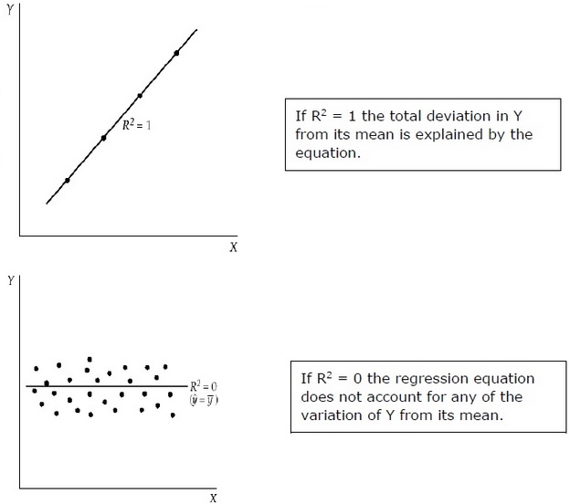
Co-efficient of Determination (R2)
Co-efficient of determination is a measure which indicates the percentage of the variation in the dependent variable is due to the variations in the independent variables. R2 is a measure of the goodness of fit model. Following are the methods −
Total Sum of Squares (TSS)
Sum of the squared deviations of the sample values of Y from the mean of Y.
TSS = SUM ( Yi − Y)2
Yi = dependent variables
Y = mean of dependent variables
i = number of observations
Regression Sum of Squares (RSS)
Sum of the squared deviations of the estimated values of Y from the mean of Y.
RSS = SUM ( i − uY)2
i = estimated value of Y
Y = mean of dependent variables
i = number of variations
Error Sum of Squares (ESS)
Sum of the squared deviations of the sample values of Y from the estimated values of Y.
ESS = SUM ( Yi − i)2
i = estimated value of Y
Yi = dependent variables
i = number of observations
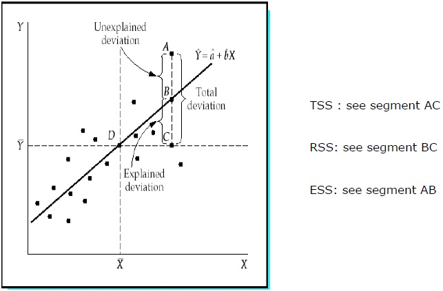
R2 measures the proportion of the total deviation of Y from its mean which is explained by the regression model. The closer the R2 is to unity, the greater the explanatory power of the regression equation. An R2 close to 0 indicates that the regression equation will have very little explanatory power.
For evaluating the regression coefficients, a sample from the population is used rather than the entire population. It is important to make assumptions about the population based on the sample and to make a judgment about how good these assumptions are.
Evaluating the Regression Coefficients
Each sample from the population generates its own intercept. To calculate the statistical difference following methods can be used −
Two tailed test −
Null Hypothesis: H0: b = 0
Alternative Hypothesis: Ha: b ≠ 0
One tailed test −
Null Hypothesis: H0: b > 0 (or b < 0)
Alternative Hypothesis: Ha: b < 0 (or b > 0)
Statistic Test −
b = estimated coefficient
E (b) = b = 0 (Null hypothesis)
SEb = Standard error of the coefficient
.Value of t depends on the degree of freedom, one or two failed test, and level of significance. To determine the critical value of t, t-table can be used. Then comes the comparison of the t-value with the critical value. One needs to reject the null hypothesis if the absolute value of the statistic test is greater than or equal to the critical t-value. Do not reject the null hypothesis, I the absolute value of the statistic test is less than the critical tvalue.
Multiple Regression Analysis
Unlike simple regression in multiple regression analysis, the coefficients indicate the change in dependent variables assuming the values of the other variables are constant.
The test of statistical significance is called F-test. The F-test is useful as it measures the statistical significance of the entire regression equation rather than just for an individual. Here In null hypothesis, there is no relationship between the dependent variable and the independent variables of the population.
The formula is − H0: b1 = b2 = b3 = . = bk = 0
No relationship exists between the dependent variable and the k independent variables for the population.
F-test static −
$$F \: =\: \frac{ \left ( \frac{R^2}{K} \right )}{\frac{(1-R^2)}{(n-k-1)}}$$
Critical value of F depends on the numerator and denominator degree of freedom and level of significance. F-table can be used to determine the critical Fvalue. In comparison to Fvalue with the critical value (F*) −
If F > F*, we need to reject the null hypothesis.
If F < F*, do not reject the null hypothesis as there is no significant relationship between the dependent variable and all independent variables.
Market System & Equilibrium
In economics, a market refers to the collective activity of buyers and sellers for a particular product or service.
The Economic Systems
Economic market system is a set of institutions for allocating resources and making choices to satisfy human wants. In a market system, the forces and interaction of supply and demand for each commodity determines what and how much to produce.
In price system, the combination is based on least combination method. This method maximizes the profit and reduces the cost. Thus firms using least combination method can lower the cost and make profit. Resources are allocated by planning. In a market economy, goods are allocated according to the decisions of producers and consumers.
Pure Capitalism − Pure capitalism market economic system is a system in which individuals own productive resources and as it is the private ownership; they can be used in any manner subject to the productive legal restrictions.
Communism − Communism is an economy in which workers are motivated to contribute to the economy. Government has most of the control in this system. The government decides what to produce, how much, and how to produce. This is an economic decision making through planned economy.
Mixed Economy − Mixed economy is a system where most of the wealth is generated by businesses and the government also plays an important role.
Demand and Supply Curves
The market demand curve indicates the maximum price that buyers will pay to purchase a given quantity of the market product.
The market supply curve indicates the minimum price that suppliers would accept to be willing to provide a given supply of the market product.
In order to have buyers and sellers agree on the quantity that would be provided and purchased, the price needs to be a right level. The market equilibrium is the quantity and associated price at which there is concurrence between sellers and buyers.
Now lets have a look at the typical supply and demand curve presentation.
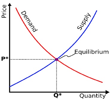
From the above graphical presentation, we can clearly see the point at which the supply and demand curves intersect with each other which we call as Equilibrium point.
Market Equilibrium
Market equilibrium is determined at the intersection of the market demand and market supply. The price that equates the quantity demanded with the quantity supplied is the equilibrium price and amount that people are willing to buy and sellers are willing to offer at the equilibrium price level is the equilibrium quantity.
A market situation in which the quantity demanded exceeds the quantity supplied shows the shortage of the market. A shortage occurs at a price below the equilibrium level. A market situation in which the quantity supplied exceeds the quantity demanded, there exists the surplus of the market. A surplus occurs at a price above the equilibrium level.
If a market is not at equilibrium, market forces try to move it equilibrium. Lets have a look − If the market price is above the equilibrium value, there is an excess of supply in the market, which means there is more supply than demand. In this situation, sellers try to reduce the price of their good to clear their inventories. They also slow down their production. The lower price helps more people to buy, which reduces the supply further. This process further results in increase in demand and decrease in supply until the market price equals the equilibrium price.
If the market price is below the equilibrium value, then there is excess in demand. In this case, buyers bid up the price of the goods. As the price goes up, some buyers tend to quit trying because they don't want to, or can't pay the higher price. Eventually, the upward pressure on price and supply will stabilize at market equilibrium.
Demand & Elasticities
The 'Law Of Demand' states that, all other factors being equal, as the price of a good or service increases, consumer demand for the good or service will decrease, and vice versa.
Demand elasticity is a measure of how much the quantity demanded will change if another factor changes.
Changes in Demand
Change in demand is a term used in economics to describe that there has been a change, or shift in, a market's total demand. This is represented graphically in a price vs. quantity plane, and is a result of more/less entrants into the market, and the changing of consumer preferences. The shift can either be parallel or nonparallel.
Extension of Demand
Other things remaining constant, when more quantity is demanded at a lower price, it is called extension of demand.
| Px | Dx | |
|---|---|---|
| 15 | 100 | Original |
| 8 | 150 | Extension |
Contraction of Demand
Other things remaining constant, when less quantity is demanded at a higher price, it is called contraction of demand.
| Px | Dx | |
|---|---|---|
| 10 | 100 | Original |
| 12 | 50 | Contraction |
Concept of Elasticity
Law of demand explains the inverse relationship between price and demand of a commodity but it does not explain to the extent to which demand of a commodity changes due to change in price.
A measure of a variable's sensitivity to a change in another variable is elasticity. In economics, elasticity refers the degree to which individuals change their demand in response to price or income changes.
It is calculated as −
Elasticity of Demand
Elasticity of Demand is the degree of responsiveness of change in demand of a commodity due to change in its prices.
Importance of Elasticity of Demand
Importance to producer − A producer has to consider elasticity of demand before fixing the price of a commodity.
Importance to government − If elasticity of demand of a product is low then government will impose heavy taxes on the production of that commodity and vice versa.
Importance in foreign market − If elasticity of demand of a produce is low in the international market then exporter can charge higher price and earn more profit.
Methods to Calculate Elasticity of Demand
Price Elasticity of demand
The price elasticity of demand is the percentage change in the quantity demanded of a good or a service, given a percentage change in its price.
Total Expenditure Method
In this, the elasticity of demand is measured with the help of total expenditure incurred by customer on purchase of a commodity.
Total Expenditure = Price per unit × Quantity Demanded
Proportionate Method or % Method
This method is an improvement over the total expenditure method in which simply the directions of elasticity could be known, i.e. more than 1, less than 1 and equal to 1. The two formulas used are −
Geometric Method
In this method, elasticity of demand can be calculated with the help of straight line curve joining both axis - x & y.
Factors Affecting Price Elasticity of Demand
The key factors which determine the price elasticity of demand are discussed below −
Substitutability
Number of substitutes available for a product or service to a consumer is an important factor in determining the price elasticity of demand. The larger the numbers of substitutes available, the greater is the price elasticity of demand at any given price.
Proportion of Income
Another important factor effecting price elasticity is the proportion of income of consumers. It is argued that larger the proportion of an individuals income, the greater is the elasticity of demand for that good at a given price.
Time
Time is also a significant factor affecting the price elasticity of demand. Generally consumers take time to adjust to the changed circumstances. The longer it takes them to adjust to a change in the price of a commodity, the lesser price elastic would be to the demand for a good or service.
Income Elasticity
Income elasticity is a measure of the relationship between a change in the quantity demanded for a commodity and a change in real income. Formula for calculating income elasticity is as follows −
Following are the Features of Income Elasticity −
If the proportion of income spent on goods remains the same as income increases, then income elasticity for the goods is equal to one.
If the proportion of income spent on goods increases as income increases, then income elasticity for the goods is greater than one.
If the proportion of income spent on goods decreases as income increases, then income elasticity for the goods is less by one.
Cross Elasticity of Demand
An economic concept that measures the responsiveness in the quantity demanded of one commodity when a change in price takes place in another good. The measure is calculated by taking the percentage change in the quantity demanded of one good, divided by the percentage change in price of the substitute good −
If two goods are perfect substitutes for each other, cross elasticity is infinite.
If two goods are totally unrelated, cross elasticity between them is zero.
If two goods are substitutes like tea and coffee, the cross elasticity is positive.
When two goods are complementary like tea and sugar to each other, the cross elasticity between them is negative.
Total Revenue (TR) and Marginal Revenue
Total revenue is the total amount of money that a firm receives from the sale of its goods. If the firm practices single pricing rather than price discrimination, then TR = total expenditure of the consumer = P × Q
Marginal revenue is the revenue generated from selling one extra unit of a good or service. It can be determined by finding the change in TR following an increase in output of one unit. MR can be both positive and negative. A revenue schedule shows the amount of revenue generated by a firm at different prices −
| Price | Quantity Demanded | Total Revenue | Marginal Revenue |
|---|---|---|---|
| 10 | 1 | 10 | |
| 9 | 2 | 18 | 8 |
| 8 | 3 | 24 | 6 |
| 7 | 4 | 28 | 4 |
| 6 | 5 | 30 | 2 |
| 5 | 6 | 30 | 0 |
| 4 | 7 | 28 | -2 |
| 3 | 8 | 24 | -4 |
| 2 | 9 | 18 | -6 |
| 1 | 10 | 10 | -8 |
Initially, as output increases total revenue also increases, but at a decreasing rate. It eventually reaches a maximum and then decreases with further output. Whereas when marginal revenue is 0, total revenue is the maximum. Increase in output beyond the point where MR = 0 will lead to a negative MR.
Price Ceiling and Price Flooring
Price ceilings and price flooring are basically price controls.
Price Ceilings
Price ceilings are set by the regulatory authorities when they believe certain commodities are sold too high of a price. Price ceilings become a problem when they are set below the market equilibrium price.
There is excess demand or a supply shortage, when the price ceilings are set below the market price. Producers dont produce as much at the lower price, while consumers demand more because the goods are cheaper. Demand outstrips supply, so there is a lot of people who want to buy at this lower price but can't.
Price Flooring
Price flooring are the prices set by the regulatory bodies for certain commodities when they believe that they are sold in an unfair market with too low prices.
Price floors are only an issue when they are set above the equilibrium price, since they have no effect if they are set below the market clearing price.
When they are set above the market price, then there is a possibility that there will be an excess supply or a surplus. If this happens, producers who can't foresee trouble ahead will produce larger quantities.
Demand Forecasting
Demand
Demand is a widely used term, and in common is considered synonymous with terms like want or 'desire'. In economics, demand has a definite meaning which is different from ordinary use. In this chapter, we will explain what demand from the consumers point of view is and analyze demand from the firm perspective.
Demand for a commodity in a market depends on the size of the market. Demand for a commodity entails the desire to acquire the product, willingness to pay for it along with the ability to pay for the same.
Law of Demand
The law of demand is one of the vital laws of economic theory. According to the law of demand, other things being equal, if the price of a commodity falls, the quantity demanded will rise and if the price of a commodity rises, its quantity demanded declines. Thus other things being constant, there is an inverse relationship between the price and demand of commodities.
Things which are assumed to be constant are income of consumers, taste and preference, price of related commodities, etc., which may influence the demand. If these factors undergo change, then this law of demand may not hold good.
Definition of Law of Demand
According to Prof. Alfred Marshall The greater the amount to be sold, the smaller must be the price at which it is offered in order that it may find purchase. Lets have a look at an illustration to further understand the price and demand relationship assuming all other factors being constant −
| Item | Price (Rs.) | Quantity Demanded (Units) |
|---|---|---|
| A | 10 | 15 |
| B | 9 | 20 |
| C | 8 | 40 |
| D | 7 | 60 |
| E | 6 | 80 |
In the above demand schedule, we can see when the price of commodity X is 10 per unit, the consumer purchases 15 units of the commodity. Similarly, when the price falls to 9 per unit, the quantity demanded increases to 20 units. Thus quantity demanded by the consumer goes on increasing until the price is lowest i.e. 6 per unit where the demand is 80 units.
The above demand schedule helps in depicting the inverse relationship between the price and quantity demanded. We can also refer the graph below to have more clear understanding of the same −
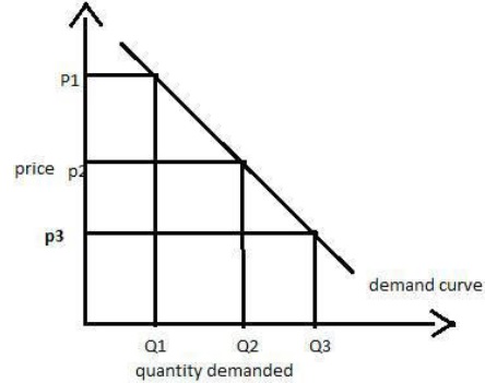
We can see from the above graph, the demand curve is sloping downwards. It can be clearly seen that when the price of the commodity rises from P3 to P2, the quantity demanded comes down Q3 to Q2.
Theory of Consumer Behavior
The demand for a commodity depends on the utility of the consumer. If a consumer gets more satisfaction or utility from a particular commodity, he would pay a higher price too for the same and vice - versa.
In economics, all human motives, desires, and wishes are called wants. Wants may arise due to any cause. Since the resources are limited, we have to choose between urgent wants and not so urgent wants. In economics wants could be classified into following three categories −
Necessities − Necessities are those wants which are essential for living. The wants without which humans cannot do anything are necessities. For example, food, clothing and shelter.
Comforts − Comforts are the commodities which are not essential for our living but are required for a happy living. For example, buying a car, air travel.
Luxuries − Luxuries are those wants which are surplus and costly. They are not essential for our living but add efficiency to our lifestyle. For example, spending on designer clothes, fine wines, antique furniture, luxury chocolates, business air travel.
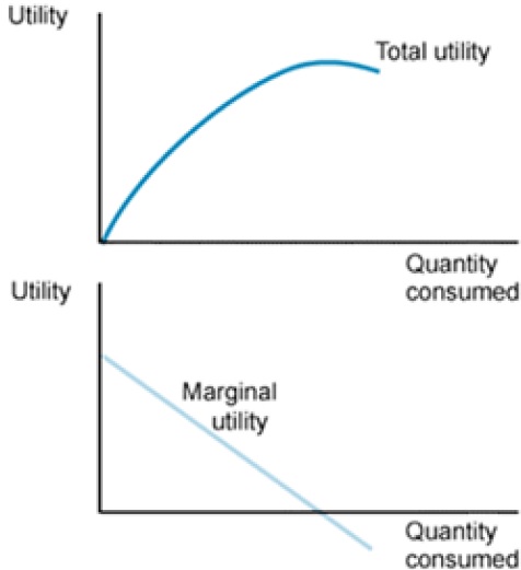
Marginal Utility Analysis
Utility is a term referring to the total satisfaction received from consuming a good or service. It differs from each individual and helps to show the satisfaction of the consumer after consumption of a commodity. In economics, utility is a measure of preferences over some set of goods and services.
Marginal Utility is formulated by Alfred Marshall, a British economist. It is the additional benefit / utility derived from the consumption of an extra unit of a commodity.
Following are the assumptions of Marginal utility analysis −
Cardinal Measurability Concept
This theory assumes that utility is a cardinal concept which means it is a measurable or quantifiable concept. This theory is quite helpful as it helps an individual to express his satisfaction in numbers by comparing different commodities.
For example − If an individual derives utility equals to 5 units from the consumption of 1 unit of commodity X and 15 units from the consumption of 1 unit of commodity Y, he can conveniently explain which commodity satisfies him more.
Consistency
This assumption is a bit unreal which says the marginal utility of money remains constant throughout when the individual spending on a particular commodity. Marginal utility is measured with the following formula −
MUnth = TUn − TUn − 1
Where, MUnth − Marginal utility of Nth unit.
TUn − Total analysis of n units
TUn − 1 − Total utility of n − 1 units.
Indifference Curve Analysis
A very well accepted approach of explaining consumers demand is indifference curve analysis. As we all know that satisfaction of a human being cannot be measured in terms of money, so an approach which could be based on consumer preferences was found out as Indifference curve analysis.
Indifference curve analysis is based on the following few assumptions −
It is assumed that the consumer is consistent in his consumption pattern. That means if he prefers a combination A to B and then B to C then he must prefer A to C for results.
Another assumption is that the consumer is capable enough of ranking the preferences according to his satisfaction level.
It is also assumed that the consumer is rational and has full knowledge about the economic environment.
An indifference curve represents all those combinations of goods and services which provide same level of satisfaction to all the consumers. It means thus all the combinations provide same level of satisfaction, the consumers can prefe them equally.
A higher indifference curve signifies a higher level of satisfaction, so a consumer tries to consume as much as possible to achieve the desired level of indifference curve. The consumer to achieve it has to work under two constraints namely − he has to pay the required price for the goods and also has to face the problem of limited money income.
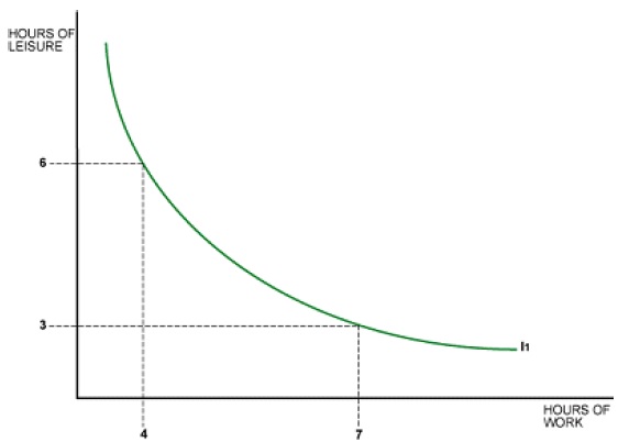
The above graph highlights that the shape of the indifference curve is not a straight line. This is due to the concept of the diminishing marginal rate of substitution between the two goods.
Consumer Equilibrium
A consumer achieves the state of equilibrium when he gets maximum satisfaction from the goods and does not have to position the goods according to their satisfaction level. Consumer equilibrium is based on the following assumptions −
Prices of the goods are fixed
Another assumption is that the consumer has fixed income which he has to spend on all the goods.
The consumer takes rational decisions to maximize his satisfaction.
Consumer equilibrium is quite superior to utility analysis as consumer equilibrium takes into consideration more than one product at a time and it also does not assume constancy of money.
A consumer achieves equilibrium when as per his income and prices of the goods he consumes, he gets maximum satisfaction. That is, when he reaches highest indifference curve possible with his budget line.
In the figure below, the consumer is in equilibrium at point H when he consumes 100 units of food and purchases 5 units of clothing. The budget line AB is tangent to the highest possible indifference curve at point H.
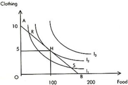
The consumer is in equilibrium at point H. He is on the highest possible indifference curve given budgetary constraint and prices of two goods.
Theory of Production
In economics, production theory explains the principles in which the business has to take decisions on how much of each commodity it sells and how much it produces and also how much of raw material ie., fixed capital and labor it employs and how much it will use. It defines the relationships between the prices of the commodities and productive factors on one hand and the quantities of these commodities and productive factors that are produced on the other hand.
Concept
Production is a process of combining various inputs to produce an output for consumption. It is the act of creating output in the form of a commodity or a service which contributes to the utility of individuals.
In other words, it is a process in which the inputs are converted into outputs.
Function
The Production function signifies a technical relationship between the physical inputs and physical outputs of the firm, for a given state of the technology.
Q = f (a, b, c, . . . . . . z)
Where a,b,c ....z are various inputs such as land, labor ,capital etc. Q is the level of the output for a firm.
If labor (L) and capital (K) are only the input factors, the production function reduces to −
Q = f(L, K)
Production Function describes the technological relationship between inputs and outputs. It is a tool that analysis the qualitative input output relationship and also represents the technology of a firm or the economy as a whole.
Production Analysis
Production analysis basically is concerned with the analysis in which the resources such as land, labor, and capital are employed to produce a firms final product. To produce these goods the basic inputs are classified into two divisions −
Variable Inputs
Inputs those change or are variable in the short run or long run are variable inputs.
Fixed Inputs
Inputs that remain constant in the short term are fixed inputs.
Cost Function
Cost function is defined as the relationship between the cost of the product and the output. Following is the formula for the same −
C = F [Q]
Cost function is divided into namely two types −
Short Run Cost
Short run cost is an analysis in which few factors are constant which wont change during the period of analysis. The output can be changed ie., increased or decreased in the short run by changing the variable factors.
Following are the basic three types of short run cost −
Long Run Cost
Long-run cost is variable and a firm adjusts all its inputs to make sure that its cost of production is as low as possible.
Long run cost = Long run variable cost
In the long run, firms dont have the liberty to reach equilibrium between supply and demand by altering the levels of production. They can only expand or reduce the production capacity as per the profits. In the long run, a firm can choose any amount of fixed costs it wants to make short run decisions.
Law of Variable Proportions
The law of variable proportions has following three different phases −
- Returns to a Factor
- Returns to a Scale
- Isoquants
In this section, we will learn more on each of them.
Returns to a Factor
Increasing Returns to a Factor
Increasing returns to a factor refers to the situation in which total output tends to increase at an increasing rate when more of variable factor is mixed with the fixed factor of production. In such a case, marginal product of the variable factor must be increasing. Inversely, marginal price of production must be diminishing.
Constant Returns to a Factor
Constant returns to a factor refers to the stage when increasing the application of the variable factor does not result in increasing the marginal product of the factor rather, marginal product of the factor tends to stabilize. Accordingly, total output increases only at a constant rate.
Diminishing Returns to a Factor
Diminishing returns to a factor refers to a situation in which the total output tends to increase at a diminishing rate when more of the variable factor is combined with the fixed factor of production. In such a situation, marginal product of the variable must be diminishing. Inversely the marginal cost of production must be increasing.
Returns to a Scale
If all inputs are changed simultaneously or proportionately, then the concept of returns to scale has to be used to understand the behavior of output. The behavior of output is studied when all the factors of production are changed in the same direction and proportion. Returns to scale are classified as follows −
Increasing returns to scale − If output increases more than proportionate to the increase in all inputs.
Constant returns to scale − If all inputs are increased by some proportion, output will also increase by the same proportion.
Decreasing returns to scale − If increase in output is less than proportionate to the increase in all inputs.
For example − If all factors of production are doubled and output increases by more than two times, then the situation is of increasing returns to scale. On the other hand, if output does not double even after a 100 per cent increase in input factors, we have diminishing returns to scale.
The general production function is Q = F (L, K)
Isoquants
Isoquants are a geometric representation of the production function. The same level of output can be produced by various combinations of factor inputs. The locus of all possible combinations is called the Isoquant.
Characteristics of Isoquant
- An isoquant slopes downward to the right.
- An isoquant is convex to origin.
- An isoquant is smooth and continuous.
- Two isoquants do not intersect.
Types of Isoquants
The production isoquant may assume various shapes depending on the degree of substitutability of factors.
Linear Isoquant
This type assumes perfect substitutability of factors of production. A given commodity may be produced by using only capital or only labor or by an infinite combination of K and L.
Input-Output Isoquant
This assumes strict complementarily, that is zero substitutability of the factors of production. There is only one method of production for any one commodity. The isoquant takes the shape of a right angle. This type of isoquant is called Leontief Isoquant.
Kinked Isoquant
This assumes limited substitutability of K and L. Generally, there are few processes for producing any one commodity. Substitutability of factors is possible only at the kinks. It is also called activity analysis-isoquant or linear-programming isoquant because it is basically used in linear programming.
Least Cost Combination of Inputs
A given level of output can be produced using many different combinations of two variable inputs. In choosing between the two resources, the saving in the resource replaced must be greater than the cost of resource added. The principle of least cost combination states that if two input factors are considered for a given output then the least cost combination will have inverse price ratio which is equal to their marginal rate of substitution.
Marginal Rate of Substitution
MRS is defined as the units of one input factor that can be substituted for a single unit of the other input factor. So MRS of x2 for one unit of x1 is −
Therefore the least cost combination of two inputs can be obtained by equating MRS with inverse price ratio.
x2 * P2 = x1 * P1
Cost & Breakeven Analysis
In managerial economics another area which is of great importance is cost of production. The cost which a firm incurs in the process of production of its goods and services is an important variable for decision making. Total cost together with total revenue determines the profit level of a business. In order to maximize profits a firm endeavors to increase its revenue and lower its costs.
Cost Concepts
Costs play a very important role in managerial decisions especially when a selection between alternative courses of action is required. It helps in specifying various alternatives in terms of their quantitative values.
Following are various types of cost concepts −
Future and Past Costs
Future costs are those costs that are likely to be incurred in future periods. Since the future is uncertain, these costs have to be estimated and cannot be expected to absolute correct figures. Future costs can be well planned, if the future costs are considered too high, management can either plan to reduce them or find out ways to meet them.
Management needs to estimate future costs for a various managerial uses where future cost are relevant such as appraisal, capital expenditure, introduction of new products, estimation of future profit and loss statement, cost control decisions, and expansion programs.
Past costs are actual costs which were incurred on the past and they are documented essentially for record keeping activity. These costs can be observed and evaluated. Past costs serve as the basis for projecting future cost but if they are regarded high, management can indulge in checks to find out the factors responsible without being able to do anything about reducing them.
Incremental and Sunk Costs
Incremental costs are defined as the change in overall costs that result from particular decision being made. Change in product line, change in output level, change in distribution channels are some examples of incremental costs. Incremental costs may include both fixed and variable costs. In the short period, incremental cost will consist of variable costcosts of additional labor, additional raw materials, power, fuel etc.
Sunk cost is the one which is not altered by a change in the level or nature of business activity. It will remain the same irrespective of activity level. Sunk costs are the expenditures that have been made in the past or must be paid in the future as a part of contractual agreement. These costs are irrelevant for decision making as they do not vary with the changes contemplated for future by the management.
Out-of-Pocket and Book Costs
Out-of-pocket costs are those that involve immediate payments to outsiders as opposed to book costs that do not require current cash expenditure"
Wages and salaries paid to the employees are out-of-pocket costs while salary of the owner manager, if not paid, is a book cost.
The interest cost of owners own fund and depreciation cost are other examples of book cost. Book costs can be converted into out-of-pocket costs by selling assets and leasing them back from the buyer.
If a factor of production is owned, its cost is a book cost while if it is hired it is an out-of-pocket cost.
Replacement and Historical Costs
Historical cost of an asset states the cost of plant, equipment, and materials at the price paid originally for them, while the replacement cost states the cost that the firm would have to incur if it wants to replace or acquire the same asset now.
For example − If the price of bronze at the time of purchase in 1973 was Rs.18 per kg and if the present price is Rs.21 per kg, the original cost Rs.18 is the historical cost while Rs.21 is the replacement cost.
Explicit Costs and ImplicitCosts
Explicit costs are those expenses which are actually paid by the firm. These costs appear in the accounting records of the firm. On the other hand, implicit costs are theoretical costs in the sense that they go unrecognized by the accounting system.
Actual Costs and Opportunity Costs
Actual costs mean the actual expenditure incurred for producing a good or service. These costs are the costs that are generally recorded in account books.
For example − Actual wages paid, cost of materials purchased.
The concept of opportunity cost is very important in modern economic analysis. The opportunity costs are the return from the second best use of the firms resources, which the firm forfeits. It avails its return from the best use of the resources.
For example, a farmer who is producing wheat can also produce potatoes with the same factors. Therefore, the opportunity cost of a ton of wheat is the amount of the output of potatoes which he gives up.
Direct Costs and Indirect Costs
There are some costs which can be directly attributed to the production of a unit for a given product. These costs are called direct costs.
Costs which cannot be separated and clearly attributed to individual units of production are classified as indirect costs.
Types of Costs
All the costs faced by companies/ business organizations can be categorized into two main types −
- Fixed costs
- Variable costs
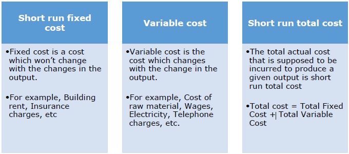
Fixed costs are expenses that have to be paid by a company, independent of any business activity. It is one of the two components of the total cost of goods or service, along with variable cost.
Examples include rent, buildings, machinery, etc.
Variable costs are corporate expenses that vary in direct proportion to the quantity of output. Unlike fixed costs, which remain constant regardless of output, variable costs are a direct function of production volume, rising whenever production expands and falling whenever it contracts.
Examples of common variable costs include raw materials, packaging, and labor directly involved in a company's manufacturing process.
Determinants of Cost
The general determinants of cost are as follows
- Output level
- Prices of factors of production
- Productivities of factors of production
- Technology
Short-Run Cost-Output Relationship
Once the firm has invested resources into the factors such as capital, equipment, building, top management personnel, and other fixed assets, their amounts cannot be changed easily. Thus in the short-run there are certain resources whose amount cannot be changed when the desired rate of output changes, those are called fixed factors.
There are other resources whose quantity used can be changed almost instantly with the output change and they are called variable factors. Since certain factors do not change with the change in output, the cost to the firm of these resources is also fixed, hence fixed cost does not vary with output. Thus, the larger the quantity produced, the lower will be the fixed cost per unit and marginal fixed cost will always be zero.
On the other hand, those factors whose quantity can be changed in the short-run is known as variable cost. Thus, the total cost of a business is the sum of its total variable costs (TVC) and total fixed cost (TFC).
TC = TFC + TVC
Long-Run Cost-Output Relationship
The long-run is a period of time during which the firm can vary all its inputs. None of the factors is fixed and all can be varied to expand output.
It is a period of time sufficiently long to permit the changes in plant like − the capital equipment, machinery, land etc., in order to expand or contract output.
The long-run cost of production is the least possible cost of production of producing any given level of output when all inputs are variable including the size of the plant. In the long-run there is no fixed factor of production and hence there is no fixed cost.
If Q = f(L, K)
TC = L. PL + K. PK
Economies and Diseconomies of Scale
Economies of Scale
As the production increases, efficiency of production also increases. The advantages of large scale production that result in lower unit costs are the reason for the economies of scale. There are two types of economies of scale −
Internal Economies of Scale
It refers to the advantages that arise as a result of the growth of the firm. When a company reduces costs and increases production, internal economies of scale are achieved. Internal economies of scale relate to lower unit costs.
External Economies of Scale
It refers to the advantages firms can gain as a result of the growth of the industry. It is normally associated with a particular area. External economies of scale occur outside of a firm and within an industry. Thus, when an industry's scope of operations expands due to the creation of a better transportation network, resulting in a decrease in cost for a company working within that industry, external economies of scale are said to have been achieved.
Diseconomies of Scale
When the prediction of economic theory becomes true that the firm may become less efficient, when it becomes too large then this theory holds true. The additional costs of becoming too large are called diseconomies of scale. Diseconomies of scale result in rising long run average costs which are experienced when a firm expands beyond its optimum scale.
For Example − Larger firms often suffer poor communication because they find it difficult to maintain an effective flow of information between departments. Time lags in the flow of information can also create problems in terms of response time to changing market condition.
Contribution and Breakeven Analysis
Break-even analysis is a very important aspect of business plan. It helps the business in determining the cost structure and the amount of sales to be done to earn profits.
It is usually included as a part of business plan to observe the profits and is enormously useful in pricing and controlling cost.
Using the above formula, the business can determine how many units it needs to produce to reach break-even.
When a firm attains break even, the cost incurred gets covered. Beyond this point, every additional unit which would be sold would result in increasing profit. The increase in profit would be by the amount of unit contribution margin.
Lets have a look at the following key terms −
Fixed costs − Costs that do not vary with output
Variable costs − Costs that vary with the quantity produced or sold.
Total cost − Fixed costs plus variable costs at level of output.
Profit − The difference between total revenue and total costs, when revenues are higher.
Loss − The difference between total revenue and total cost, when cost is higher than the revenue.
Breakeven chart
The Break-even analysis chart is a graphical representation of costs at various levels of activity.
With this, business managers are able to ascertain the period when there is neither profit nor loss made for the organization. This is commonly known as "Break-even Point".
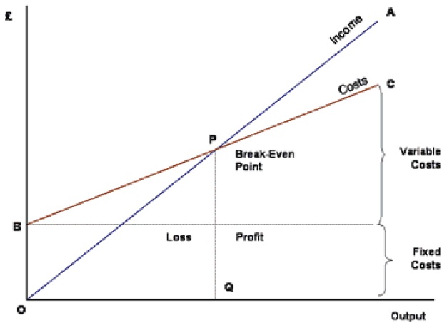
In the graph above, the line OA represents the variation of income at various levels of production activity.
OB represents the total fixed costs in the business. As output increases, variable costs are incurred, which means fixed + variable cost also increase. At low levels of output, costs are greater than income.
At the point of intersection P (Break even Point) , costs are exactly equal to income, and hence neither profit nor loss is made.
Market Structure & Pricing Decisions
Price determination is one of the most crucial aspects in economics. Business managers are expected to make perfect decisions based on their knowledge and judgment. Since every economic activity in the market is measured as per price, it is important to know the concepts and theories related to pricing. Pricing discusses the rationale and assumptions behind pricing decisions. It analyzes unique market needs and discusses how business managers reach upon final pricing decisions.
It explains the equilibrium of a firm and is the interaction of the demand faced by the firm and its supply curve. The equilibrium condition differs under perfect competition, monopoly, monopolistic competition, and oligopoly. Time element is of great relevance in the theory of pricing since one of the two determinants of price, namely supply depends on the time allowed to it for adjustment.
Market Structure
A market is the area where buyers and sellers contact each other and exchange goods and services. Market structure is said to be the characteristics of the market. Market structures are basically the number of firms in the market that produce identical goods and services. Market structure influences the behavior of firms to a great extent. The market structure affects the supply of different commodities in the market.
When the competition is high there is a high supply of commodity as different companies try to dominate the markets and it also creates barriers to entry for the companies that intend to join that market. A monopoly market has the biggest level of barriers to entry while the perfectly competitive market has zero percent level of barriers to entry. Firms are more efficient in a competitive market than in a monopoly structure.
Perfect Competition
Perfect competition is a situation prevailing in a market in which buyers and sellers are so numerous and well informed that all elements of monopoly are absent and the market price of a commodity is beyond the control of individual buyers and sellers
With many firms and a homogeneous product under perfect competition no individual firm is in a position to influence the price of the product that means price elasticity of demand for a single firm will be infinite.
Pricing Decisions
Determinants of Price Under Perfect Competition
Market price is determined by the equilibrium between demand and supply in a market period or very short run. The market period is a period in which the maximum that can be supplied is limited by the existing stock. The market period is so short that more cannot be produced in response to increased demand. The firms can sell only what they have already produced. This market period may be an hour, a day or a few days or even a few weeks depending upon the nature of the product.
Market Price of a Perishable Commodity
In the case of perishable commodity like fish, the supply is limited by the available quantity on that day. It cannot be stored for the next market period and therefore the whole of it must be sold away on the same day whatever the price may be.
Market Price of Non-Perishable and Reproducible Goods
In case of non-perishable but reproducible goods, some of the goods can be preserved or kept back from the market and carried over to the next market period. There will then be two critical price levels.
The first, if price is very high the seller will be prepared to sell the whole stock. The second level is set by a low price at which the seller would not sell any amount in the present market period, but will hold back the whole stock for some better time. The price below which the seller will refuse to sell is called the Reserve Price.
Monopolistic Competition
Monopolistic competition is a form of market structure in which a large number of independent firms are supplying products that are slightly differentiated from the point of view of buyers. Thus, the products of the competing firms are close but not perfect substitutes because buyers do not regard them as identical. This situation arises when the same commodity is being sold under different brand names, each brand being slightly different from the others.
For example − Lux, Liril, Dove, etc.
Each firm is therefore the sole producer of a particular brand or product. It is monopolist as far as a particular brand is concerned. However, since the various brands are close substitutes, a large number of monopoly producers of these brands are involved in a keen competition with one another. This type of market structure, where there is competition among a large number of monopolists is called monopolistic competition.
In addition to product differentiation, the other three basic characteristics of monopolistic competition are −
There are large number of independent sellers and buyers in the market.
The relative market shares of all sellers are insignificant and more or less equal. That is, seller-concentration in the market is almost non-existent.
There are neither any legal nor any economic barriers against the entry of new firms into the market. New firms are free to enter the market and existing firms are free to leave the market.
In other words, product differentiation is the only characteristic that distinguishes monopolistic competition from perfect competition.
Monopoly
Monopoly is said to exist when one firm is the sole producer or seller of a product which has no close substitutes. According to this definition, there must be a single producer or seller of a product. If there are many producers producing a product, either perfect competition or monopolistic competition will prevail depending upon whether the product is homogeneous or differentiated.
On the other hand, when there are few producers, oligopoly is said to exist. A second condition which is essential for a firm to be called monopolist is that no close substitutes for the product of that firm should be available.
From above it follows that for the monopoly to exist, following things are essential −
One and only one firm produces and sells a particular commodity or a service.
There are no rivals or direct competitors of the firm.
No other seller can enter the market for whatever reasons legal, technical, or economic.
Monopolist is a price maker. He tries to take the best of whatever demand and cost conditions exist without the fear of new firms entering to compete away his profits.
The concept of market power applies to an individual enterprise or to a group of enterprises acting collectively. For the individual firm, it expresses the extent to which the firm has discretion over the price that it charges. The baseline of zero market power is set by the individual firm that produces and sells a homogeneous product alongside many other similar firms that all sell the same product.
Since all of the firms sell the identical product, the individual sellers are not distinctive. Buyers care solely about finding the seller with the lowest price.
In this context of perfect competition, all firms sell at an identical price that is equal to their marginal costs and no individual firm possess any market power. If any firm were to raise its price slightly above the market-determined price, it would lose all of its customers and if a firm were to reduce its price slightly below the market price, it would be swamped with customers who switch from the other firms.
Accordingly, the standard definition for market power is to define it as the divergence between price and marginal cost, expressed relative to price. In Mathematical terms we may define it as −
Oligopoly
In an oligopolistic market there are small number of firms so that sellers are conscious of their interdependence. The competition is not perfect, yet the rivalry among firms is high. Given that there are large number of possible reactions of competitors, the behavior of firms may assume various forms. Thus there are various models of oligopolistic behavior, each based on different reactions patterns of rivals.
Oligopoly is a situation in which only a few firms are competing in the market for a particular commodity. The distinguishing characteristics of oligopoly are such that neither the theory of monopolistic competition nor the theory of monopoly can explain the behavior of an oligopolistic firm.
Two of the main characteristics of Oligopoly are briefly explained below −
Under oligopoly the number of competing firms being small, each firm controls an important proportion of the total supply. Consequently, the effect of a change in the price or output of one firm upon the sales of its rival firms is noticeable and not insignificant. When any firm takes an action its rivals will in all probability react to it. The behavior of oligopolistic firms is interdependent and not independent or atomistic as is the case under perfect or monopolistic competition.
Under oligopoly new entry is difficult. It is neither free nor barred. Hence the condition of entry becomes an important factor determining the price or output decisions of oligopolistic firms and preventing or limiting entry of an important objective.
For Example − Aircraft manufacturing, in some countries: wireless communication, media, and banking.
Managerial Economics - Pricing Strategies
Pricing is the process of determining what a company will receive in exchange for its product or service. A business can use a variety of pricing strategies when selling a product or service. The price can be set to maximize profitability for each unit sold or from the market overall. It can be used to defend an existing market from new entrants, to increase market share within a market or to enter a new market.
There is a need to follow certain guidelines in pricing of the new product. Following are the common pricing strategies −
Pricing a New Product
Most companies do not consider pricing strategies in a major way, on a day-today basis. The marketing of a new product poses a problem because new products have no past information.
Fixing the first price of the product is a major decision. The future of the company depends on the soundness of the initial pricing decision of the product. In large multidivisional companies, top management needs to establish specific criteria for acceptance of new product ideas.
The price fixed for the new product must have completed the advanced research and development, satisfy public criteria such as consumer safety and earn good profits. In pricing a new product, below mentioned two types of pricing can be selected −
Skimming Price
Skimming price is known as short period device for pricing. Here, companies tend to charge higher price in initial stages. Initial high helps to Skim the Cream of the market as the demand for new product is likely to be less price elastic in the early stages.
Penetration Price
Penetration price is also referred as stay out price policy since it prevents competition to a great extent. In penetration pricing lowest price for the new product is charged. This helps in prompt sales and keeping the competitors away from the market. It is a long term pricing strategy and should be adopted with great caution.
Multiple Products
As the name indicates multiple products signifies production of more than one product. The traditional theory of price determination assumes that a firm produces a single homogenous product. But firms in reality usually produce more than one product and then there exists interrelationships between those products. Such products are joint products or multiproducts. In joint products the inputs are common in the production process and in multi-products the inputs are independent but have common overhead expenses. Following are the pricing methods followed −
Full Cost Pricing Method
Full cost plus pricing is a price-setting method under which you add together the direct material cost, direct labor cost, selling and administrative cost, and overhead costs for a product and add to it a markup percentage in order to derive the price of the product. The pricing formula is −
This method is most commonly used in situations where products and services are provided based on the specific requirements of the customer. Thus, there is reduced competitive pressure and no standardized product being provided. The method may also be used to set long-term prices that are sufficiently high to ensure a profit after all costs have been incurred.
Marginal Cost Pricing Method
The practice of setting the price of a product to equal the extra cost of producing an extra unit of output is called marginal pricing in economics. By this policy, a producer charges for each product unit sold, only the addition to total cost resulting from materials and direct labor. Businesses often set prices close to marginal cost during periods of poor sales.
For example, an item has a marginal cost of $2.00 and a normal selling price is $3.00, the firm selling the item might wish to lower the price to $2.10 if demand has waned. The business would choose this approach because the incremental profit of 10 cents from the transaction is better than no sale at all.
Transfer Pricing
Transfer Pricing relates to international transactions performed between related parties and covers all sorts of transactions.
The most common being distributorship, R&D, marketing, manufacturing, loans, management fees, and IP licensing.
All intercompany transactions must be regulated in accordance with applicable law and comply with the "arm's length" principle which requires holding an updated transfer pricing study and an intercompany agreement based upon the study.
Some corporations perform their intercompany transactions based upon previously issued studies or an ill advice they have received, to work at a cost plus X%. This is not sufficient, such a decision has to be supported in terms of methodology and the amount of overhead by a proper transfer pricing study and it has to be updated each financial year.
Dual Pricing
In simple words, different prices offered for the same product in different markets is dual pricing. Different prices for same product are basically known as dual pricing. The objective of dual pricing is to enter different markets or a new market with one product offering lower prices in foreign county.
There are industry specific laws or norms which are needed to be followed for dual pricing. Dual pricing strategy does not involve arbitrage. It is quite commonly followed in developing countries where local citizens are offered the same products at a lower price for which foreigners are paid more.
Airline Industry could be considered as a prime example of Dual Pricing. Companies offer lower prices if tickets are booked well in advance. The demand of this category of customers is elastic and varies inversely with price.
As the time passes the flight fares start increasing to get high prices from the customers whose demands are inelastic. This is how companies charge different fare for the same flight tickets. The differentiating factor here is the time of booking and not nationality.
Price Effect
Price effect is the change in demand in accordance to the change in price, other things remaining constant. Other things include − Taste and preference of the consumer, income of the consumer, price of other goods which are assumed to be constant. Following is the formula for price effect −
Price effect is the summation of two effects, substitution effect and income effect
Price effect = Substitution effect − Income effect
Substitution Effect
In this effect the consumer is compelled to choose a product that is less expensive so that his satisfaction is maximized, as the normal income of the consumer is fixed. It can be explained with the below examples −
Consumers will buy less expensive foods such as vegetables over meat.
Consumers could buy less amount of meat to keep expenses in control.
Income Effect
Change in demand of goods based on the change in consumers discretionary income. Income effect comprises of two types of commodities or products −
Normal goods − If there is a price fall, demand increases as real income increases and vice versa.
Inferior goods − In case of inferior goods, demand increases due to an increase in the real income.
Investment Under Certainty
Capital Budgeting is the process by which the firm decides which long-term investments to make. Capital Budgeting projects, i.e., potential long-term investments, are expected to generate cash flows over several years.
Capital Budgeting also explains the decisions in which all the incomes and expenditures are covered. These decisions involve all inflows and outflows of funds of an undertaking for a particular period of time.
Capital Budgeting techniques under certainty can be divided into the following two groups −
Non Discounted Cash Flow
- Pay Back Period
- Accounting Rate of Return (ARR)
Discounted Cash Flow
- Net Present Value (NPV)
- Profitability Index (PI)
- Internal Rate of Return (IRR)
The payback period (PBP) is the traditional method of capital budgeting. It is the simplest and perhaps the most widely used quantitative method for appraising capital expenditure decision; i.e. it is the number of years required to recover the original cash outlay invested in a project.
Non-Discounted Cash Flow
Non-discounted cash flow techniques are also known as traditional techniques.
Pay Back Period
Payback period is one of the traditional methods of budgeting. It is widely used as quantitative method and is the simplest method in capital expenditure decision. Payback period helps in analyzing the number of years required to recover the original cash outlay invested in a particular project. The formula widely used to calculate payback period is −
Advantages of Using PBP
PBP is a cost effective and easy to calculate method. It is simple to use and does not require much of the time for calculation. It is more helpful for short term earnings.
Accounting Rate of Return (ARR)
The ARR is the ratio after tax profit divided by the average investment. ARR is also known as return on investment method (ROI). Following formula is usually used to calculate ARR −
The average profits after tax are obtained by adding up the profit after tax for each year and dividing the result by the number of years.
Advantages of Using ARR
ARR is simple to use and as it is based on accounting information, it is easily available. ARR is usually used as a performance evaluation measure and not as a decision making tool as it does not use cash flow information.
Discounted Cash Flow Techniques
Discounted cash flow techniques consider time value of money and are therefore also known as modern techniques.
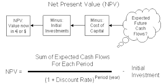
Net Present Value (NPV)
The net present value is one of the discounted cash flow techniques. It is the difference between the present value of future cash inflows and the present value of the initial outlay, discounted at the firms cost of capital. It recognizes the cash flow streams at different time intervals and can be computed only when they are expressed in terms of common denominator (present value). Present value is calculated by determining an appropriate discount rate. NPV is calculated with the help of equation.
NPV = Present value of cash inflows − Initial investment.
Advantages
NPV is considered as the most appropriate measure of profitability. It considers all the years of cash flow, and recognizes the time value for money. It is an absolute measure of profitability that means it gives output in terms of absolute amount. The NPVs of the projects can be added together which is not possible in other methods.
Profitability Index (PI)
Profitability index method is also known as benefit cost ratio as numerator measures benefits and denominator measures cost like the NPV approach. It is the ratio obtained by dividing the present value of future cash inflows by the present value of cash outlays. Mathematically it is defined as −
Advantages
In a capital rationing situation, PI is a better evaluation method as compared to NPV method. It considers the time value of money along cash flows generated by the project.
| Present Cash Value | |||
|---|---|---|---|
| Year | Cash Flows | @ 5% Discount | @ 10% Discount |
| 0 | $ -10,000.00 | $ -10,000.00 | $ -10,000.00 |
| 1 | $ 2,000.00 | $ 1,905.00 | $ 1,818.00 |
| 2 | $ 2,000.00 | $ 1,814.00 | $ 1,653.00 |
| 3 | $ 2,000.00 | $ 1,728.00 | $ 1,503.00 |
| 4 | $ 2,000.00 | $ 1,645.00 | $ 1,366.00 |
| 5 | $ 5,000.00 | $ 3,918.00 | $ 3,105.00 |
| Total | $ 1,010.00 | $ -555.00 | |
Internal Rate of Return (IRR)
Internal rate of return is also known as yield on investment. IRR depends entirely on the initial outlay of the projects which are evaluated. It is the compound annual rate of return that the firm earns, if it invests in the project and receives the given cash inflows. Mathematically IRR is determined by the following equation −
Where,
R = The internal rate of return
Ct = Cash inflows at t period
C0 = Initial investment
Example −
| Internal Rate of Return | |
|---|---|
| Opening Balance | -100,000 |
| Year 1 Cash Flow | 110000 |
| Year 2 Cash Flow | 113000 |
| Year 3 Cash Flow | 117000 |
| Year 4 Cash Flow | 120000 |
| Year 5 Cash Flow | 122000 |
| Proceeds from Sale | 1100000 |
| IRR | 9.14% |
Advantages
IRR considers the total cash flows generated by a project over the life of the project. It measures profitability of the projects in percentage and can be easily compared with the opportunity cost of capital. It also considers the time value of money.
Investment Under Uncertainty
Macroeconomics is a part of economic study which analyzes the economy as a whole. It is the average of the entire economy and does not study any individual unit or a firm. It studies the national income, total employment, aggregate demand and supply etc.
Nature of Macroeconomics
Macroeconomics is basically known as theory of income. It is concerned with the problems of economic fluctuations, unemployment, inflation or deflation and economic growth. It deals with the aggregates of all quantities not with individual price levels or outputs but with national output.
As per G. Ackley, Macroeconomics concerns itself with such variables −
- Aggregate volume of the output of an economy
- Extent to which resources are employed
- Size of the national income
- General price level
Scope of Macroeconomics
Macroeconomics is much of theoretical and practical importance. Following are the points covered under the scope of macroeconomics −
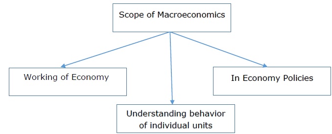
Working of the Economy
The study of macroeconomics is crucial to understand the working of an economy. Economic problems are mainly related to the employment, behavior of total income and general price in the economy. Macroeconomics help in making the elimination process more understandable.
In Economy Policies
Macroeconomics is very useful in an economic policy. Underdeveloped economies face innumerable problems related to overpopulation, inflation, balance of payments etc. The main responsibilities of government are controlling the overpopulation, prices, volume of trade etc.
Following are the economic problems where macroeconomics study are useful −
- In national income
- In unemployment
- In economic growth
- In monetary problems
Understanding the Behavior of Individual Units
The demand for individual products depends upon aggregate demand in the economy therefore understanding the behavior of individual units is very important in macroeconomics. Firstly, to solve the problem of deficiency in demand of individual products, understanding the causes of fall in aggregate demand is required. Similarly to know the reasons for increase in costs of a particular firm or industry, it is first required to understand the average cost conditions of the whole economy. Thus, the study of individual units is not possible without macroeconomics.
Macroeconomics enhances our knowledge of the functioning of an economy by studying the behavior of national income, output, savings, and consumptions.
Circular Flow Model of Economy
Circular flow model is the basic economic model and it describes the flow of money and products throughout the economy in a very simplified manner. This model divides the market into two categories −
- Market of goods and services
- Market for factor of production
The circular flow diagram displays the relationship of resources and money between firms and households. Every adult individual understands its basic structure from personal experience. Firms employ workers, who spend their income on goods produced by the firms. This money is then used to compensate the workers and buy raw materials to make the goods. This is the basic structure behind the circular flow diagram. Lets have a look at the following diagram −
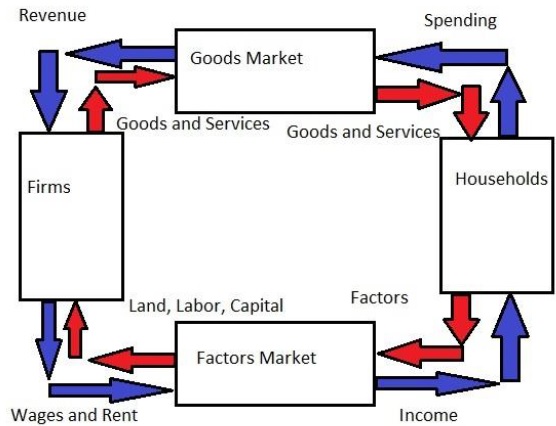
In the above model, we can see that the firms and the households interact with each other in both product market as well as factor of production market. The product market is the market where all the products by the firms are exchanged and factors of production market is where inputs such as land, labor, capital and resources are exchanged. Households sell their resources to the businesses in the factor market to earn money. The prices of the resources, the businesses purchase are costs. Business produces goods utilizing the resources provided by the households, which are then sold in the product market. Households use their incomes to purchase these goods in the product market. In return for the goods, businesses bring in revenue.
National Income & Measurement
Definition of National Income
The total net value of all goods and services produced within a nation over a specified period of time, representing the sum of wages, profits, rents, interest, and pension payments to residents of the nation.
Measures of National Income
For the purpose of measurement and analysis, national income can be viewed as an aggregate of various component flows. The most comprehensive measure of aggregate income which is widely known is Gross National Product at market prices.
Gross and Net Concept
Gross emphasizes that no allowance for capital consumption has been made or that depreciation has yet to be deducted. Net indicates that provision for capital consumption has already been made or that depreciation has already been deducted.
National and Domestic Concepts
The term national denotes that the aggregate under consideration represents the total income which accrues to the normal residents of a country due to their participation in world production during the current year.
It is also possible to measure the value of the total output or income originating within the specified geographical boundary of a country known as domestic territory. The resulting measure is called "domestic product".
Market Prices and Factor Costs
The valuation of the national product at market prices indicates the total amount actually paid by the final buyers while the valuation of national product at factor cost is a measure of the total amount earned by the factors of production for their contribution to the final output.
GNP at market price = GNP at factor cost + indirect taxes - Subsidies.
NNP at market price = NNP at factor cost + indirect taxes - Subsidies
Gross National Product and Gross Domestic Product
For some purposes we need to find the total income generated from production within the territorial boundaries of an economy irrespective of whether it belongs to the inhabitants of that nation or not. Such an income is known as Gross Domestic Product (GDP) and found as −
GDP = GNP - Nnet Factor Income From Abroad
Net Factor Income from Abroad = Factor Income Received From Abroad - Factor Income Paid Abroad
Net National Product
The NNP is an alternative and closely related measure of the national income. It differs from GNP in only one respect. GNP is the sum of final products. It includes consumption of goods, gross investment, government expenditures on goods and services, and net exports.
GNP = NNP − Depreciation
NNP includes net private investment while GNP includes gross private domestic investment.
Personal Income
Personal income is calculated by subtracting from national income those types of incomes which are earned but not received and adding those types which are received but not currently earned.
Personal Income = NNP at Factor Cost − Undistributed Profits − Corporate Taxes + Transfer Payments
Disposable Income
Disposable income is the total income that actually remains with individuals to dispose off as they wish. It differs from personal income by the amount of direct taxes paid by individuals.
Disposable Income = Personal Income − Personal taxes
Value Added
The concept of value added is a useful device to find out the exact amount that is added at each stage of production to the value of the final product. Value added can be defined as the difference between the value of output produced by that firm and the total expenditure incurred by it on the materials and intermediate products purchased from other business firms.
Methods of Measuring National Income
Lets have a look at the following ways of measuring national income −
Product Approach
In product approach, national income is measured as a flow of goods and services. Value of money for all final goods and services is produced in an economy during a year. Final goods are those goods which are directly consumed and not used in further production process. In our economy product approach benefits various sectors like forestry, agriculture, mining etc to estimate gross and net value.
Income Approach
In income approach, national income is measured as a flow of factor incomes. Income received by basic factors like labor, capital, land and entrepreneurship are summed up. This approach is also called as income distributed approach.
Expenditure Approach
This method is known as the final product method. In this method, national income is measured as a flow of expenditure incurred by the society in a particular year. The expenditures are classified as personal consumption expenditure, net domestic investment, government expenditure on goods and services and net foreign investment.
These three approaches to the measurement of national income yield identical results. They provide three alternative methods of measuring essentially the same magnitude.
National Income Determination
Factors Determining the National Income
According to Keynes there are two major factors that determine the national income of an economy −
Aggregate Supply
Aggregate supply comprises of consumer goods as well as producer goods. It is defined as total value of goods and services produced and supplied at a particular point of time. When goods and services produced at a particular point of time is multiplied by the respective prices of goods and services, it helps us in getting the total value of the national output. The formula for determining the aggregate national income is follows −
Aggregate Income = Consumption(C) + Saving (S)
Few factor prices such as wages, rents are rigid in the short run. When demand in an economy increases, firms also tend to increase production to some extent. However, along with the production, some factor prices and the amount of inputs needed to increase production also increase.
Aggregate Demand
Aggregate demand is the effective aggregate expenditure of an economy in a particular time period. It is the effective demand which is equal to the actual expenditure. Aggregate demand involves concepts namely aggregate demand for consumer goods and aggregate demand for capital goods. Aggregate demand can be represented by the following formula −
AD = C + I
As per Keynes theory of nation income, investment (I) remains constant throughout, while consumption (C) keeps changing, and thus consumption is the major determinant of income.
Modern Theories of Economic Growth
Definition of Economic Growth
Economic growth refers to an increase in the goods and services produced by an economy over a particular period of time. It is measured as a percentage increase in real gross domestic product which is GDP adjusted to inflation. GDP is the market value for all the final goods and services produced in an economy.
Theories of Economic Growth
The Classical Approach
Adam Smith laid emphasis on increasing returns as a source of economic growth. He focused on foreign trade to widen the market and raise productivity of trading countries. Trade enables a country to buy goods from abroad at a lower cost as compared to which they can be produced in the home country.
In modern growth theory, Lucas has strongly emphasized the role of increasing returns through direct foreign investment which encourages learning by doing through knowledge capital. In Southeast Asia, the newly industrialized countries (NICs) have achieved very high growth rates in the last two decades.
The Neoclassical Approach
The neoclassical approach to economic growth has been divided into two sections −
The first section is the competitive model of Walrasian equilibrium where markets play a very crucial role in allocating the resources effectively. To secure the optimal allocation of inputs and outputs, markets for labor, finance and capital have been used. This type of competitive paradigm was used by Solow to develop a growth model.
The second section of the neoclassical model assumes that technology is given. Solow used the interpretation that technology in the production function is superficial. The point is that R&D investment and human capital through learning by doing were not explicitly recognized.
The neoclassical growth model developed by Solow fails to explain the fact of actual growth behavior. This failure is caused due to the models prediction that per capita output approaches a steady state path along which it grows at a rate that is given. This means that the long-term rate of national growth is determined outside the model and is independent of preferences and most aspects of the production function and policy measures.
The Modern Approach
The modern approach to market comprises of several features. The new economy emerging today is spreading all over the world. It is a revolution in knowledge capital and information explosion. Following are the important key elements −
Innovation theory by Schumpeter, inter firm and inter industry diffusion of knowledge.
Increasing efficiency of the telecommunications and micro-computer industry.
Global expansion of trade through modern externalities and networks.
Modern theory of economic growth focuses mainly on two channels of inducing growth through expenses spent on research and development on the core component of knowledge innovations. First channel is the impact on the available goods and services and the other one is the impact on the stock of knowledge phenomena.
Business Cycles & Stabilization
Business cycles are the rhythmic fluctuations in the aggregate level of economic activity of a nation. Business cycle comprises of following phases −
- Depression
- Recovery
- Prosperity
- Inflation
- Recession
Business cycles occur because of reasons such as good or bad climatic conditions, under consumption or over consumption, strikes, war, floods, draughts, etc
Theories of Business Cycles
Schumpeters Theory of Innovation
According to Schumpeter, an innovation is defined as the development of a new product or introduction of a new product or a process of production, development of new market or a change in the market.
Over − Investment Theory
Professor Hayek says, primary cause of business cycles is monetary overestimate. He says business cycles are caused by over investment and consequently by over production. When a bank charges rate of interest below the equilibrium rate, the business has to borrow more funds which leads to business fluctuations.
Monetary Theory
According to Professor Hawtrey, all the changes in the business cycles take place due to monetary policies. According to him the flow in the monetary demand leads to prosperity or depression in the economy. Cyclical fluctuations are caused by expansion and contraction of bank credit. These conditions increase or decrease the flow of money in the economy.
Stabilization Policies
Stabilization policies are also known as counter cycle policies. These policies try to counter the natural ups and downs of business cycles. Expansionary stabilization policies are useful to reduce unemployment during contraction and contractionary policies are used to reduce inflation during expansion.
Instruments of Stabilization Policies
The flow chart of stablilization policies is described below:
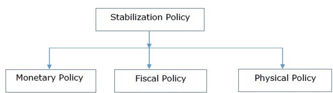
Monetary Policy
Monetary policy is employed by the government as an effective tool to promote economic stability and achieve certain predetermined objectives. It deals with the total money supply and its management in an economy. Objectives of monetary policy include exchange rate stability, price stability, full employment, rapid economic growth, etc.
Fiscal Policy
Fiscal policy helps to formulate rational consumption policy and helps to increase savings. It raises the volume of investments and the standards of living. Fiscal policy creates more jobs, reduces economic inequalities and controls, inflation and deflation. Fiscal policy as an instrument to fight depression and create full employment conditions is much more effective as compared to monetary policy.
Physical Policy
When monetary policy and fiscal policy are inadequate to control prices, government adapts physical policy. These policies can be introduced swiftly and thus the result is quite rapid. Theses controls are more discriminatory as compared to monetary policy. They tend to vary effectively in the intensity of the operation of control from time to time in various sectors.
Inflation & ITS Control Measures
Inflation
In economics, inflation means rise in the general level of prices of goods and services over a period of time in an economy. Inflation may affect the economy either in positive way or negative way.
Causes of Inflation
The causes of inflation are as follows −
Inflation may occur sometimes due to excessive bank credit or currency depreciation.
It may be caused due to increase in demand in relation to supply of all types goods and services due to a rapid increase in population.
Inflation also may be also be caused by a change in the value of production costs of goods.
Export boom inflation also comes into existence when a considerable increase in exports may cause a shortage in the home country.
Inflation is also caused by decrease in supplies, consumer confidence, and corporate decisions to charge more.
Measures to Control Inflation
There are many ways of controlling inflation in an economy −
Monetary Measure
The most important method of controlling inflation is monetary policy of the Central Bank. Most central banks use high interest rates as a way to fight inflation. Following are the monetary measures used to control inflation −
Bank Rate Policy − Bank rate policy is the most common tool against inflation. The increase in bank rate increases the cost of borrowings which reduces commercial banks borrowing from the central bank.
Cash Reserve Ratio − To control inflation, the central bank needs to raise CRR which helps in reducing the lending capacity of the commercial banks.
Open Market Operations − Open market operations mean the sale and purchase of government securities and bonds by the central bank.
Fiscal Policy
Fiscal measures are another important set of measures to control inflation which include taxation, public borrowings, and government expenses. Some of the fiscal measures to control inflation are as follows −
- Increase in savings
- Increase in taxes
- Surplus budgets
Wage and Price Controls
Wage and price controls help in controlling wages as the price increases. Price control and wage control is a short term measure but is successful; since in long run, it controls inflation along with rationing.
Impact of Inflation on Managerial Decision Making
Inflation is of course the all too familiar problem of too much money (demand) chasing too few goods (supply), with the upshot of prices and expectations everywhere tending to rise higher and higher.
The Role of a Manager
In these circumstance, a business manager has to take appropriate decisions and measures based on macro economic uncertainties like inflation and the occasional recession.
A true test of a business manager lies in delivering profitability ie., the extent to which he increases revenues and also reduces costs even during economic uncertainties.
In the current scenario, they are supposed to get faster solutions to the problems of coping with soaring prices (for example) by understanding the process of how inflation distorts the traditional functions of money along with recommendations.
The Effect of Management
The bottom-line impact is that, Customers / clients reward efficient management with profits and penalize inefficient management with losses. Hence, it is advisable to be well prepared to tackle these areas.