- Managerial Economics - Home
- Managerial Economics Overview
- Business Firms & Decisions
- Economic Analysis & Optimizations
- Regression Technique
- Production & Cost Analysis
- Theory of Production
- Cost & Breakeven Analysis
- Market Structure & Pricing Theory
- Market Structure & Pricing Decisions
- Pricing Strategies
- Capital Budgeting
- Investment Under Certainty
- Investment Under Uncertainty
- Macroeconomic Aspects
- Macroeconomics Basics
- Circular Flow Model of Economy
- National Income & Measurement
- National Income Determination
- Theories of Economic Growth
- Business Cycles & Stabilization
- Inflation & ITS Control Measures
- Managerial Economics Resources
- Managerial Economics - Quick Guide
- Managerial Economics - Resources
- Managerial Economics - Discussion
Demand Forecasting
Demand
Demand is a widely used term, and in common is considered synonymous with terms like want or 'desire'. In economics, demand has a definite meaning which is different from ordinary use. In this chapter, we will explain what demand from the consumers point of view is and analyze demand from the firm perspective.
Demand for a commodity in a market depends on the size of the market. Demand for a commodity entails the desire to acquire the product, willingness to pay for it along with the ability to pay for the same.
Law of Demand
The law of demand is one of the vital laws of economic theory. According to the law of demand, other things being equal, if the price of a commodity falls, the quantity demanded will rise and if the price of a commodity rises, its quantity demanded declines. Thus other things being constant, there is an inverse relationship between the price and demand of commodities.
Things which are assumed to be constant are income of consumers, taste and preference, price of related commodities, etc., which may influence the demand. If these factors undergo change, then this law of demand may not hold good.
Definition of Law of Demand
According to Prof. Alfred Marshall The greater the amount to be sold, the smaller must be the price at which it is offered in order that it may find purchase. Lets have a look at an illustration to further understand the price and demand relationship assuming all other factors being constant −
| Item | Price (Rs.) | Quantity Demanded (Units) |
|---|---|---|
| A | 10 | 15 |
| B | 9 | 20 |
| C | 8 | 40 |
| D | 7 | 60 |
| E | 6 | 80 |
In the above demand schedule, we can see when the price of commodity X is 10 per unit, the consumer purchases 15 units of the commodity. Similarly, when the price falls to 9 per unit, the quantity demanded increases to 20 units. Thus quantity demanded by the consumer goes on increasing until the price is lowest i.e. 6 per unit where the demand is 80 units.
The above demand schedule helps in depicting the inverse relationship between the price and quantity demanded. We can also refer the graph below to have more clear understanding of the same −
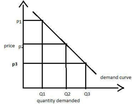
We can see from the above graph, the demand curve is sloping downwards. It can be clearly seen that when the price of the commodity rises from P3 to P2, the quantity demanded comes down Q3 to Q2.
Theory of Consumer Behavior
The demand for a commodity depends on the utility of the consumer. If a consumer gets more satisfaction or utility from a particular commodity, he would pay a higher price too for the same and vice - versa.
In economics, all human motives, desires, and wishes are called wants. Wants may arise due to any cause. Since the resources are limited, we have to choose between urgent wants and not so urgent wants. In economics wants could be classified into following three categories −
Necessities − Necessities are those wants which are essential for living. The wants without which humans cannot do anything are necessities. For example, food, clothing and shelter.
Comforts − Comforts are the commodities which are not essential for our living but are required for a happy living. For example, buying a car, air travel.
Luxuries − Luxuries are those wants which are surplus and costly. They are not essential for our living but add efficiency to our lifestyle. For example, spending on designer clothes, fine wines, antique furniture, luxury chocolates, business air travel.
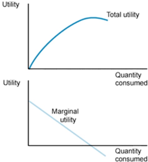
Marginal Utility Analysis
Utility is a term referring to the total satisfaction received from consuming a good or service. It differs from each individual and helps to show the satisfaction of the consumer after consumption of a commodity. In economics, utility is a measure of preferences over some set of goods and services.
Marginal Utility is formulated by Alfred Marshall, a British economist. It is the additional benefit / utility derived from the consumption of an extra unit of a commodity.
Following are the assumptions of Marginal utility analysis −
Cardinal Measurability Concept
This theory assumes that utility is a cardinal concept which means it is a measurable or quantifiable concept. This theory is quite helpful as it helps an individual to express his satisfaction in numbers by comparing different commodities.
For example − If an individual derives utility equals to 5 units from the consumption of 1 unit of commodity X and 15 units from the consumption of 1 unit of commodity Y, he can conveniently explain which commodity satisfies him more.
Consistency
This assumption is a bit unreal which says the marginal utility of money remains constant throughout when the individual spending on a particular commodity. Marginal utility is measured with the following formula −
MUnth = TUn − TUn − 1
Where, MUnth − Marginal utility of Nth unit.
TUn − Total analysis of n units
TUn − 1 − Total utility of n − 1 units.
Indifference Curve Analysis
A very well accepted approach of explaining consumers demand is indifference curve analysis. As we all know that satisfaction of a human being cannot be measured in terms of money, so an approach which could be based on consumer preferences was found out as Indifference curve analysis.
Indifference curve analysis is based on the following few assumptions −
It is assumed that the consumer is consistent in his consumption pattern. That means if he prefers a combination A to B and then B to C then he must prefer A to C for results.
Another assumption is that the consumer is capable enough of ranking the preferences according to his satisfaction level.
It is also assumed that the consumer is rational and has full knowledge about the economic environment.
An indifference curve represents all those combinations of goods and services which provide same level of satisfaction to all the consumers. It means thus all the combinations provide same level of satisfaction, the consumers can prefe them equally.
A higher indifference curve signifies a higher level of satisfaction, so a consumer tries to consume as much as possible to achieve the desired level of indifference curve. The consumer to achieve it has to work under two constraints namely − he has to pay the required price for the goods and also has to face the problem of limited money income.
The above graph highlights that the shape of the indifference curve is not a straight line. This is due to the concept of the diminishing marginal rate of substitution between the two goods.
Consumer Equilibrium
A consumer achieves the state of equilibrium when he gets maximum satisfaction from the goods and does not have to position the goods according to their satisfaction level. Consumer equilibrium is based on the following assumptions −
Prices of the goods are fixed
Another assumption is that the consumer has fixed income which he has to spend on all the goods.
The consumer takes rational decisions to maximize his satisfaction.
Consumer equilibrium is quite superior to utility analysis as consumer equilibrium takes into consideration more than one product at a time and it also does not assume constancy of money.
A consumer achieves equilibrium when as per his income and prices of the goods he consumes, he gets maximum satisfaction. That is, when he reaches highest indifference curve possible with his budget line.
In the figure below, the consumer is in equilibrium at point H when he consumes 100 units of food and purchases 5 units of clothing. The budget line AB is tangent to the highest possible indifference curve at point H.
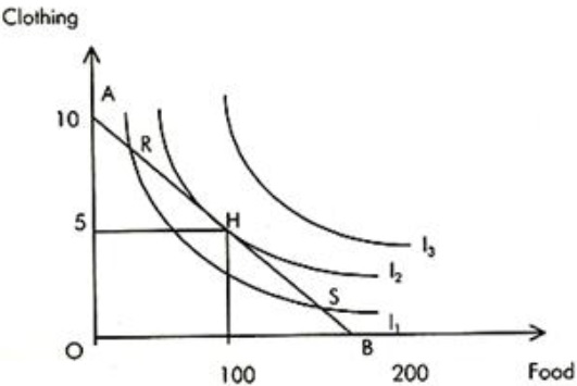
The consumer is in equilibrium at point H. He is on the highest possible indifference curve given budgetary constraint and prices of two goods.