Convex Optimization - Quick Guide

---

---

Convex Optimization - Introduction

This course is useful for the students who want to solve non-linear optimization problems that arise in various engineering and scientific applications. This course starts with basic theory of linear programming and will introduce the concepts of convex sets and functions and related terminologies to explain various theorems that are required to solve the non linear programming problems. This course will introduce various algorithms that are used to solve such problems. These type of problems arise in various applications including machine learning, optimization problems in electrical engineering, etc. It requires the students to have prior knowledge of high school maths concepts and calculus.

In this course, the students will learn to solve the optimization problems like $min f\left ( x \right )$ subject to some constraints.

These problems are easily solvable if the function $f\left ( x \right )$ is a linear function and if the constraints are linear. Then it is called a linear programming problem (LPP). But if the constraints are non-linear, then it is difficult to solve the above problem. Unless we can plot the functions in a graph, then try to analyse the optimization can be one way, but we can't plot a function if it's beyond three dimensions. Hence there comes the techniques of non-linear programming or convex programming to solve such problems. In these tutorial, we will focus on learning such techniques and in the end, a few algorithms to solve such problems. first we will bring the notion of convex sets which is the base of the convex programming problems. Then with the introduction of convex functions, we will some important theorems to solve these problems and some algorithms based on these theorems.

Terminologies

• The space $\mathbb{R}^n$ − It is an n-dimensional vector with real numbers, defined as follows − $\mathbb{R}^n=\left \{ \left ( x_1,x_2,...,x_n \right )^{\tau }:x_1,x_2,....,x_n \in \mathbb{R} \right \}$

• The space $\mathbb{R}^{mXn}$ − It is a set of all real values matrices of order $mXn$.

Convex Optimization - Linear Programming

Methodology

Linear Programming also called Linear Optimization, is a technique which is used to solve mathematical problems in which the relationships are linear in nature. the basic nature of Linear Programming is to maximize or minimize an objective function with subject to some constraints. The objective function is a linear function which is obtained from the mathematical model of the problem. The constraints are the conditions which are imposed on the model and are also linear.

• From the given question, find the objective function.
• find the constraints.
• Draw the constraints on a graph.
• find the feasible region, which is formed by the intersection of all the constraints.
• find the vertices of the feasible region.
• find the value of the objective function at these vertices.
• The vertice which either maximizes or minimizes the objective function (according to the question) is the answer.

Examples

Step 1 − Maximize $5x+3y$ subject to

$x+y\leq 2$,

$3x+y\leq 3$,

$x\geq 0 \:and \:y\geq 0$

Solution −

The first step is to find the feasible region on a graph.

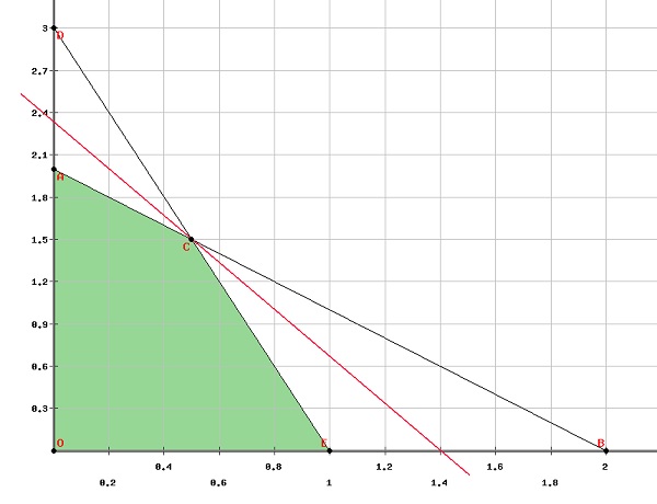
Clearly from the graph, the vertices of the feasible region are

$\left ( 0, 0 \right )\left ( 0, 2 \right )\left ( 1, 0 \right )\left ( \frac{1}{2}, \frac{3}{2} \right )$

Let $f\left ( x, y \right )=5x+3y$

Putting these values in the objective function, we get −

$f\left ( 0, 0 \right )$=0

$f\left ( 0, 2 \right )$=6

$f\left ( 1, 0 \right )$=5

$f\left ( \frac{1}{2}, \frac{3}{2} \right )$=7

Therefore, the function maximizes at $\left ( \frac{1}{2}, \frac{3}{2} \right )$

Step 2 − A watch company produces a digital and a mechanical watch. Long-term projections indicate an expected demand of at least 100 digital and 80 mechanical watches each day. Because of limitations on production capacity, no more than 200 digital and 170 mechanical watches can be made daily. To satisfy a shipping contract, a total of at least 200 watches much be shipped each day.

If each digital watch sold results in a $\$2$ loss, but each mechanical watch produces a $\$5$ profit, how many of each type should be made daily to maximize net profits?

Solution −

Let $x$ be the number of digital watches produced

$y$ be the number of mechanical watches produced

According to the question, at least 100 digital watches are to be made daily and maximaum 200 digital watches can be made.

$\Rightarrow 100 \leq \:x\leq 200$

Similarly, at least 80 mechanical watches are to be made daily and maximum 170 mechanical watches can be made.

$\Rightarrow 80 \leq \:y\leq 170$

Since at least 200 watches are to be produced each day.

$\Rightarrow x +y\leq 200$

Since each digital watch sold results in a $\$2$ loss, but each mechanical watch produces a $\$5$ profit,

Total profit can be calculated as

$Profit =-2x + 5y$

And we have to maximize the profit, Therefore, the question can be formulated as −

Maximize $-2x + 5y$ subject to

$100 \:\leq x\:\leq 200$

$80 \:\leq y\:\leq 170$

$x+y\:\leq 200$

Plotting the above equations in a graph, we get,

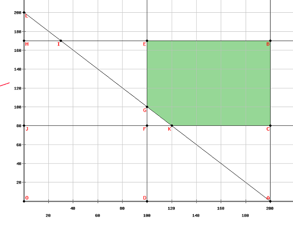
The vertices of the feasible region are

$\left ( 100, 170\right )\left ( 200, 170\right )\left ( 200, 180\right )\left ( 120, 80\right ) and \left ( 100, 100\right )$

The maximum value of the objective function is obtained at $\left ( 100, 170\right )$ Thus, to maximize the net profits, 100 units of digital watches and 170 units of mechanical watches should be produced.

Convex Optimization - Norm

A norm is a function that gives a strictly positive value to a vector or a variable.

Norm is a function $f:\mathbb{R}^n\rightarrow \mathbb{R}$

The basic characteristics of a norm are −

Let $X$ be a vector such that $X\in \mathbb{R}^n$

• $\left \| x \right \|\geq 0$

• $\left \| x \right \|= 0 \Leftrightarrow x= 0\forall x \in X$

• $\left \|\alpha x \right \|=\left | \alpha \right |\left \| x \right \|\forall \:x \in X and \:\alpha \:is \:a \:scalar$

• $\left \| x+y \right \|\leq \left \| x \right \|+\left \| y \right \| \forall x,y \in X$

• $\left \| x-y \right \|\geq \left \| \left \| x \right \|-\left \| y \right \| \right \|$

By definition, norm is calculated as follows −

• $\left \| x \right \|_1=\displaystyle\sum\limits_{i=1}^n\left | x_i \right |$

• $\left \| x \right \|_2=\left ( \displaystyle\sum\limits_{i=1}^n\left | x_i \right |^2 \right )^{\frac{1}{2}}$

• $\left \| x \right \|_p=\left ( \displaystyle\sum\limits_{i=1}^n\left | x_i \right |^p \right )^{\frac{1}{p}},1 \leq p \leq \infty$

Norm is a continuous function.

Proof

By definition, if $x_n\rightarrow x$ in $X\Rightarrow f\left ( x_n \right )\rightarrow f\left ( x \right ) $ then $f\left ( x \right )$ is a constant function.

Let $f\left ( x \right )=\left \| x \right \|$

Therefore, $\left | f\left ( x_n \right )-f\left ( x \right ) \right |=\left | \left \| x_n \right \| -\left \| x \right \|\right |\leq \left | \left | x_n-x \right | \:\right |$

Since $x_n \rightarrow x$ thus, $\left \| x_n-x \right \|\rightarrow 0$

Therefore $\left | f\left ( x_n \right )-f\left ( x \right ) \right |\leq 0\Rightarrow \left | f\left ( x_n \right )-f\left ( x \right ) \right |=0\Rightarrow f\left ( x_n \right )\rightarrow f\left ( x \right )$

Hence, norm is a continuous function.

Convex Optimization - Inner Product

Inner product is a function which gives a scalar to a pair of vectors.

Inner Product − $f:\mathbb{R}^n \times \mathbb{R}^n\rightarrow \kappa$ where $\kappa$ is a scalar.

The basic characteristics of inner product are as follows −

Let $X \in \mathbb{R}^n$

• $\left \langle x,x \right \rangle\geq 0, \forall x \in X$

• $\left \langle x,x \right \rangle=0\Leftrightarrow x=0, \forall x \in X$

• $\left \langle \alpha x,y \right \rangle=\alpha \left \langle x,y \right \rangle,\forall \alpha \in \kappa \: and\: \forall x,y \in X$

• $\left \langle x+y,z \right \rangle =\left \langle x,z \right \rangle +\left \langle y,z \right \rangle, \forall x,y,z \in X$

• $\left \langle \overline{y,x} \right \rangle=\left ( x,y \right ), \forall x, y \in X$

Note −

• Relationship between norm and inner product: $\left \| x \right \|=\sqrt{\left ( x,x \right )}$

• $\forall x,y \in \mathbb{R}^n,\left \langle x,y \right \rangle=x_1y_1+x_2y_2+...+x_ny_n$

Examples

1. find the inner product of $x=\left ( 1,2,1 \right )\: and \: y=\left ( 3,-1,3 \right )$

Solution

$\left \langle x,y \right \rangle =x_1y_1+x_2y_2+x_3y_3$

$\left \langle x,y \right \rangle=\left ( 1\times3 \right )+\left ( 2\times-1 \right )+\left ( 1\times3 \right )$

$\left \langle x,y \right \rangle=3+\left ( -2 \right )+3$

$\left \langle x,y \right \rangle=4$

2. If $x=\left ( 4,9,1 \right ),y=\left ( -3,5,1 \right )$ and $z=\left ( 2,4,1 \right )$, find $\left ( x+y,z \right )$

Solution

As we know, $\left \langle x+y,z \right \rangle=\left \langle x,z \right \rangle+\left \langle y,z \right \rangle$

$\left \langle x+y,z \right \rangle=\left ( x_1z_1+x_2z_2+x_3z_3 \right )+\left ( y_1z_1+y_2z_2+y_3z_3 \right )$

$\left \langle x+y,z \right \rangle=\left \{ \left ( 4\times 2 \right )+\left ( 9\times 4 \right )+\left ( 1\times1 \right ) \right \}+$

$\left \{ \left ( -3\times2 \right )+\left ( 5\times4 \right )+\left ( 1\times 1\right ) \right \}$

$\left \langle x+y,z \right \rangle=\left ( 8+36+1 \right )+\left ( -6+20+1 \right )$

$\left \langle x+y,z \right \rangle=45+15$

$\left \langle x+y,z \right \rangle=60$

Convex Optimization - Minima and Maxima

Local Minima or Minimize

$\bar{x}\in \:S$ is said to be local minima of a function $f$ if $f\left ( \bar{x} \right )\leq f\left ( x \right ),\forall x \in N_\varepsilon \left ( \bar{x} \right )$ where $N_\varepsilon \left ( \bar{x} \right )$ means neighbourhood of $\bar{x}$, i.e., $N_\varepsilon \left ( \bar{x} \right )$ means $\left \| x-\bar{x} \right \|< \varepsilon$

Local Maxima or Maximizer

$\bar{x}\in \:S$ is said to be local maxima of a function $f$ if $f\left ( \bar{x} \right )\geq f\left ( x \right ), \forall x \in N_\varepsilon \left ( \bar{x} \right )$ where $N_\varepsilon \left ( \bar{x} \right )$ means neighbourhood of $\bar{x}$, i.e., $N_\varepsilon \left ( \bar{x} \right )$ means $\left \| x-\bar{x} \right \|< \varepsilon$

Global minima

$\bar{x}\in \:S$ is said to be global minima of a function $f$ if $f\left ( \bar{x} \right )\leq f\left ( x \right ), \forall x \in S$

Global maxima

$\bar{x}\in \:S$ is said to be global maxima of a function $f$ if $f\left ( \bar{x} \right )\geq f\left ( x \right ), \forall x \in S$

Examples

Step 1 − find the local minima and maxima of $f\left ( \bar{x} \right )=\left | x^2-4 \right |$

Solution −

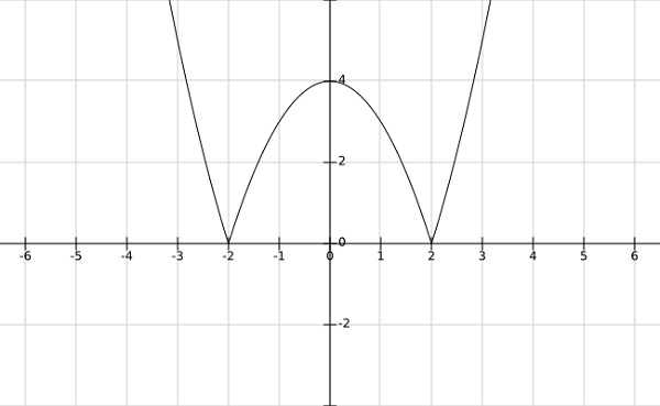
From the graph of the above function, it is clear that the local minima occurs at $x= \pm 2$ and local maxima at $x = 0$

Step 2 − find the global minima af the function $f\left (x \right )=\left | 4x^3-3x^2+7 \right |$

Solution −

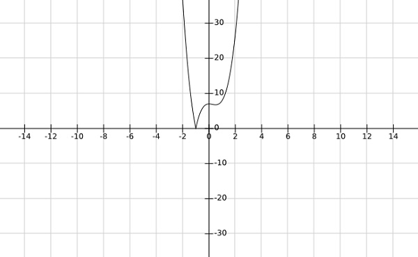
From the graph of the above function, it is clear that the global minima occurs at $x=-1$.

Convex Optimization - Convex Set

Let $S\subseteq \mathbb{R}^n$ A set S is said to be convex if the line segment joining any two points of the set S also belongs to the S, i.e., if $x_1,x_2 \in S$, then $\lambda x_1+\left ( 1-\lambda \right )x_2 \in S$ where $\lambda \in\left ( 0,1 \right )$.

Note −

• The union of two convex sets may or may not be convex.
• The intersection of two convex sets is always convex.

Proof

Let $S_1$ and $S_2$ be two convex set.

Let $S_3=S_1 \cap S_2$

Let $x_1,x_2 \in S_3$

Since $S_3=S_1 \cap S_2$ thus $x_1,x_2 \in S_1$and $x_1,x_2 \in S_2$

Since $S_i$ is convex set, $\forall$ $i \in 1,2,$

Thus $\lambda x_1+\left ( 1-\lambda \right )x_2 \in S_i$ where $\lambda \in \left ( 0,1 \right )$

Therfore, $\lambda x_1+\left ( 1-\lambda \right )x_2 \in S_1\cap S_2$

$\Rightarrow \lambda x_1+\left ( 1-\lambda \right )x_2 \in S_3$

Hence, $S_3$ is a convex set.

• Weighted average of the form $\displaystyle\sum\limits_{i=1}^k \lambda_ix_i$,where $\displaystyle\sum\limits_{i=1}^k \lambda_i=1$ and $\lambda_i\geq 0,\forall i \in \left [ 1,k \right ]$ is called conic combination of $x_1,x_2,....x_k.$

• Weighted average of the form $\displaystyle\sum\limits_{i=1}^k \lambda_ix_i$, where $\displaystyle\sum\limits_{i=1}^k \lambda_i=1$ is called affine combination of $x_1,x_2,....x_k.$

• Weighted average of the form $\displaystyle\sum\limits_{i=1}^k \lambda_ix_i$ is called linear combination of $x_1,x_2,....x_k.$

Examples

Step 1 − Prove that the set $S=\left \{ x \in \mathbb{R}^n:Cx\leq \alpha \right \}$ is a convex set.

Solution

Let $x_1$ and $x_2 \in S$

$\Rightarrow Cx_1\leq \alpha$ and $\:and \:Cx_2\leq \alpha$

To show:$\:\:y=\left ( \lambda x_1+\left ( 1-\lambda \right )x_2 \right )\in S \:\forall \:\lambda \in\left ( 0,1 \right )$

$Cy=C\left ( \lambda x_1+\left ( 1-\lambda \right )x_2 \right )=\lambda Cx_1+\left ( 1-\lambda \right )Cx_2$

$\Rightarrow Cy\leq \lambda \alpha+\left ( 1-\lambda \right )\alpha$

$\Rightarrow Cy\leq \alpha$

$\Rightarrow y\in S$

Therefore, $S$ is a convex set.

Step 2 − Prove that the set $S=\left \{ \left ( x_1,x_2 \right )\in \mathbb{R}^2:x_{1}^{2}\leq 8x_2 \right \}$ is a convex set.

Solution

Let $x,y \in S$

Let $x=\left ( x_1,x_2 \right )$ and $y=\left ( y_1,y_2 \right )$

$\Rightarrow x_{1}^{2}\leq 8x_2$ and $y_{1}^{2}\leq 8y_2$

To show − $\lambda x+\left ( 1-\lambda \right )y\in S\Rightarrow \lambda \left ( x_1,x_2 \right )+\left (1-\lambda \right )\left ( y_1,y_2 \right ) \in S\Rightarrow \left [ \lambda x_1+\left ( 1- \lambda)y_2] \in S\right ) \right ]$

$Now, \left [\lambda x_1+\left ( 1-\lambda \right )y_1 \right ]^{2}=\lambda ^2x_{1}^{2}+\left ( 1-\lambda \right )^2y_{1}^{2}+2 \lambda\left ( 1-\lambda \right )x_1y_1$

But $2x_1y_1\leq x_{1}^{2}+y_{1}^{2}$

Therefore,

$\left [ \lambda x_1 +\left ( 1-\lambda \right )y_1\right ]^{2}\leq \lambda ^2x_{1}^{2}+\left ( 1- \lambda \right )^2y_{1}^{2}+2 \lambda\left ( 1- \lambda \right )\left ( x_{1}^{2}+y_{1}^{2} \right )$

$\Rightarrow \left [ \lambda x_1+\left ( 1-\lambda \right )y_1 \right ]^{2}\leq \lambda x_{1}^{2}+\left ( 1- \lambda \right )y_{1}^{2}$

$\Rightarrow \left [ \lambda x_1+\left ( 1-\lambda \right )y_1 \right ]^{2}\leq 8\lambda x_2+8\left ( 1- \lambda \right )y_2$

$\Rightarrow \left [ \lambda x_1+\left ( 1-\lambda \right )y_1 \right ]^{2}\leq 8\left [\lambda x_2+\left ( 1- \lambda \right )y_2 \right ]$

$\Rightarrow \lambda x+\left ( 1- \lambda \right )y \in S$

Step 3 − Show that a set $S \in \mathbb{R}^n$ is convex if and only if for each integer k, every convex combination of any k points of $S$ is in $S$.

Solution

Let $S$ be a convex set. then, to show;

$c_1x_1+c_2x_2+.....+c_kx_k \in S, \displaystyle\sum\limits_{1}^k c_i=1,c_i\geq 0, \forall i \in 1,2,....,k$

Proof by induction

For $k=1,x_1 \in S, c_1=1 \Rightarrow c_1x_1 \in S$

For $k=2,x_1,x_2 \in S, c_1+c_2=1$ and Since S is a convex set

$\Rightarrow c_1x_1+c_2x_2 \in S.$

Let the convex combination of m points of S is in S i.e.,

$c_1x_1+c_2x_2+...+c_mx_m \in S,\displaystyle\sum\limits_{1}^m c_i=1 ,c_i \geq 0, \forall i \in 1,2,...,m$

Now, Let $x_1,x_2....,x_m,x_{m+1} \in S$

Let $x=\mu_1x_1+\mu_2x_2+...+\mu_mx_m+\mu_{m+1}x_{m+1}$

Let $x=\left ( \mu_1+\mu_2+...+\mu_m \right )\frac{\mu_1x_1+\mu_2x_2+\mu_mx_m}{\mu_1+\mu_2+.........+\mu_m}+\mu_{m+1}x_{m+1}$

Let $y=\frac{\mu_1x_1+\mu_2x_2+...+\mu_mx_m}{\mu_1+\mu_2+.........+\mu_m}$

$\Rightarrow x=\left ( \mu_1+\mu_2+...+\mu_m \right )y+\mu_{m+1}x_{m+1}$

Now $y \in S$ because the sum of the coefficients is 1.

$\Rightarrow x \in S$ since S is a convex set and $y,x_{m+1} \in S$

Hence proved by induction.

Convex Optimization - affine Set

A set $A$ is said to be an affine set if for any two distinct points, the line passing through these points lie in the set $A$.

Note −

• $S$ is an affine set if and only if it contains every affine combination of its points.

• Empty and singleton sets are both affine and convex set.

  For example, solution of a linear equation is an affine set.

Proof

Let S be the solution of a linear equation.

By definition, $S=\left \{ x \in \mathbb{R}^n:Ax=b \right \}$

Let $x_1,x_2 \in S\Rightarrow Ax_1=b$ and $Ax_2=b$

To prove : $A\left [ \theta x_1+\left ( 1-\theta \right )x_2 \right ]=b, \forall \theta \in\left ( 0,1 \right )$

$A\left [ \theta x_1+\left ( 1-\theta \right )x_2 \right ]=\theta Ax_1+\left ( 1-\theta \right )Ax_2=\theta b+\left ( 1-\theta \right )b=b$

Thus S is an affine set.

Theorem

If $C$ is an affine set and $x_0 \in C$, then the set $V= C-x_0=\left \{ x-x_0:x \in C \right \}$ is a subspace of C.

Proof

Let $x_1,x_2 \in V$

To show: $\alpha x_1+\beta x_2 \in V$ for some $\alpha,\beta$

Now, $x_1+x_0 \in C$ and $x_2+x_0 \in C$ by definition of V

Now, $\alpha x_1+\beta x_2+x_0=\alpha \left ( x_1+x_0 \right )+\beta \left ( x_2+x_0 \right )+\left ( 1-\alpha -\beta \right )x_0$

But $\alpha \left ( x_1+x_0 \right )+\beta \left ( x_2+x_0 \right )+\left ( 1-\alpha -\beta \right )x_0 \in C$ because C is an affine set.

Therefore, $\alpha x_1+\beta x_2 \in V$

Hence proved.

Convex Optimization - Hull

The convex hull of a set of points in S is the boundary of the smallest convex region that contain all the points of S inside it or on its boundary.

OR

Let $S\subseteq \mathbb{R}^n$ The convex hull of S, denoted $Co\left ( S \right )$ by is the collection of all convex combination of S, i.e., $x \in Co\left ( S \right )$ if and only if $x \in \displaystyle\sum\limits_{i=1}^n \lambda_ix_i$, where $\displaystyle\sum\limits_{1}^n \lambda_i=1$ and $\lambda_i \geq 0 \forall x_i \in S$

Remark − Conves hull of a set of points in S in the plane defines a convex polygon and the points of S on the boundary of the polygon defines the vertices of the polygon.

Theorem $Co\left ( S \right )= \left \{ x:x=\displaystyle\sum\limits_{i=1}^n \lambda_ix_i,x_i \in S, \displaystyle\sum\limits_{i=1}^n \lambda_i=1,\lambda_i \geq 0 \right \}$ Show that a convex hull is a convex set.

Proof

Let $x_1,x_2 \in Co\left ( S \right )$, then $x_1=\displaystyle\sum\limits_{i=1}^n \lambda_ix_i$ and $x_2=\displaystyle\sum\limits_{i=1}^n \lambda_\gamma x_i$ where $\displaystyle\sum\limits_{i=1}^n \lambda_i=1, \lambda_i\geq 0$ and $\displaystyle\sum\limits_{i=1}^n \gamma_i=1,\gamma_i\geq0$

For $\theta \in \left ( 0,1 \right ),\theta x_1+\left ( 1-\theta \right )x_2=\theta \displaystyle\sum\limits_{i=1}^n \lambda_ix_i+\left ( 1-\theta \right )\displaystyle\sum\limits_{i=1}^n \gamma_ix_i$

$\theta x_1+\left ( 1-\theta \right )x_2=\displaystyle\sum\limits_{i=1}^n \lambda_i \theta x_i+\displaystyle\sum\limits_{i=1}^n \gamma_i\left ( 1-\theta \right )x_i$

$\theta x_1+\left ( 1-\theta \right )x_2=\displaystyle\sum\limits_{i=1}^n\left [ \lambda_i\theta +\gamma_i\left ( 1-\theta \right ) \right ]x_i$

Considering the coefficients,

$\displaystyle\sum\limits_{i=1}^n\left [ \lambda_i\theta +\gamma_i\left ( 1-\theta \right ) \right ]=\theta \displaystyle\sum\limits_{i=1}^n \lambda_i+\left ( 1-\theta \right )\displaystyle\sum\limits_{i=1}^n\gamma_i=\theta +\left ( 1-\theta \right )=1$

Hence, $\theta x_1+\left ( 1-\theta \right )x_2 \in Co\left ( S \right )$

Thus, a convex hull is a convex set.

Caratheodory Theorem

Let S be an arbitrary set in $\mathbb{R}^n$.If $x \in Co\left ( S \right )$, then $x \in Co\left ( x_1,x_2,....,x_n,x_{n+1} \right )$.

Proof

Since $x \in Co\left ( S\right )$, then $x$ is representated by a convex combination of a finite number of points in S, i.e.,

$x=\displaystyle\sum\limits_{j=1}^k \lambda_jx_j,\displaystyle\sum\limits_{j=1}^k \lambda_j=1, \lambda_j \geq 0$ and $x_j \in S, \forall j \in \left ( 1,k \right )$

If $k \leq n+1$, the result obtained is obviously true.

If $k \geq n+1$, then $\left ( x_2-x_1 \right )\left ( x_3-x_1 \right ),....., \left ( x_k-x_1 \right )$ are linearly dependent.

$\Rightarrow \exists \mu _j \in \mathbb{R}, 2\leq j\leq k$ (not all zero) such that $\displaystyle\sum\limits_{j=2}^k \mu _j\left ( x_j-x_1 \right )=0$

Define $\mu_1=-\displaystyle\sum\limits_{j=2}^k \mu _j$, then $\displaystyle\sum\limits_{j=1}^k \mu_j x_j=0, \displaystyle\sum\limits_{j=1}^k \mu_j=0$

where not all $\mu_j's$ are equal to zero. Since $\displaystyle\sum\limits_{j=1}^k \mu_j=0$, at least one of the $\mu_j > 0,1 \leq j \leq k$

Then, $x=\displaystyle\sum\limits_{1}^k \lambda_j x_j+0$

$x=\displaystyle\sum\limits_{1}^k \lambda_j x_j- \alpha \displaystyle\sum\limits_{1}^k \mu_j x_j$

$x=\displaystyle\sum\limits_{1}^k\left ( \lambda_j- \alpha\mu_j \right )x_j $

Choose $\alpha$ such that $\alpha=min\left \{ \frac{\lambda_j}{\mu_j}, \mu_j\geq 0 \right \}=\frac{\lambda_j}{\mu _j},$ for some $i=1,2,...,k$

If $\mu_j\leq 0, \lambda_j-\alpha \mu_j\geq 0$

If $\mu_j> 0, then \:\frac{\lambda _j}{\mu_j}\geq \frac{\lambda_i}{\mu _i}=\alpha \Rightarrow \lambda_j-\alpha \mu_j\geq 0, j=1,2,...k$

In particular, $\lambda_i-\alpha \mu_i=0$, by definition of $\alpha$

$x=\displaystyle\sum\limits_{j=1}^k \left ( \lambda_j- \alpha\mu_j\right )x_j$,where

$\lambda_j- \alpha\mu_j\geq0$ and $\displaystyle\sum\limits_{j=1}^k\left ( \lambda_j- \alpha\mu_j\right )=1$ and $\lambda_i- \alpha\mu_i=0$

Thus, x can be representated as a convex combination of at most (k-1) points.

This reduction process can be repeated until x is representated as a convex combination of (n+1) elements.

Convex Optimization - Weierstrass Theorem

Let S be a non empty, closed and bounded set (also called compact set) in $\mathbb{R}^n$ and let $f:S\rightarrow \mathbb{R} $ be a continuous function on S, then the problem min $\left \{ f\left ( x \right ):x \in S \right \}$ attains its minimum.

Proof

Since S is non-empty and bounded, there exists a lower bound.

$\alpha =Inf\left \{ f\left ( x \right ):x \in S \right \}$

Now let $S_j=\left \{ x \in S:\alpha \leq f\left ( x \right ) \leq \alpha +\delta ^j\right \} \forall j=1,2,...$ and $\delta \in \left ( 0,1 \right )$

By the definition of infimium, $S_j$ is non-empty, for each $j$.

Choose some $x_j \in S_j$ to get a sequence $\left \{ x_j \right \}$ for $j=1,2,...$

Since S is bounded, the sequence is also bounded and there is a convergent subsequence $\left \{ y_j \right \}$, which converges to $\hat{x}$. Hence $\hat{x}$ is a limit point and S is closed, therefore, $\hat{x} \in S$. Since f is continuous, $f\left ( y_i \right )\rightarrow f\left ( \hat{x} \right )$.

Since $\alpha \leq f\left ( y_i \right )\leq \alpha+\delta^k, \alpha=\displaystyle\lim_{k\rightarrow \infty}f\left ( y_i \right )=f\left ( \hat{x} \right )$

Thus, $\hat{x}$ is the minimizing solution.

Remarks

There are two important necessary conditions for Weierstrass Theorem to hold. These are as follows −

• Step 1 − The set S should be a bounded set.

  Consider the function f\left ( x \right )=x$.

  It is an unbounded set and it does have a minima at any point in its domain.

  Thus, for minima to obtain, S should be bounded.

• Step 2 − The set S should be closed.

  Consider the function $f\left ( x \right )=\frac{1}{x}$ in the domain \left ( 0,1 \right ).

  This function is not closed in the given domain and its minima also does not exist.

  Hence, for minima to obtain, S should be closed.

Convex Optimization - Closest Point Theorem

Let S be a non-empty closed convex set in $\mathbb{R}^n$ and let $y\notin S$, then $\exists$ a point $\bar{x}\in S$ with minimum distance from y, i.e.,$\left \| y-\bar{x} \right \| \leq \left \| y-x \right \| \forall x \in S.$

Furthermore, $\bar{x}$ is a minimizing point if and only if $\left ( y-\hat{x} \right )^{T}\left ( x-\hat{x} \right )\leq 0$ or $\left ( y-\hat{x}, x-\hat{x} \right )\leq 0$

Proof

Existence of closest point

Since $S\ne \phi,\exists$ a point $\hat{x}\in S$ such that the minimum distance of S from y is less than or equal to $\left \| y-\hat{x} \right \|$.

Define $\hat{S}=S \cap \left \{ x:\left \| y-x \right \|\leq \left \| y-\hat{x} \right \| \right \}$

Since $ \hat{S}$ is closed and bounded, and since norm is a continuous function, then by Weierstrass theorem, there exists a minimum point $\hat{x} \in S$ such that $\left \| y-\hat{x} \right \|=Inf\left \{ \left \| y-x \right \|,x \in S \right \}$

Uniqueness

Suppose $\bar{x} \in S$ such that $\left \| y-\hat{x} \right \|=\left \| y-\hat{x} \right \|= \alpha$

Since S is convex, $\frac{\hat{x}+\bar{x}}{2} \in S$

But, $\left \| y-\frac{\hat{x}-\bar{x}}{2} \right \|\leq \frac{1}{2}\left \| y-\hat{x} \right \|+\frac{1}{2}\left \| y-\bar{x} \right \|=\alpha$

It can't be strict inequality because $\hat{x}$ is closest to y.

Therefore, $\left \| y-\hat{x} \right \|=\mu \left \| y-\hat{x} \right \|$, for some $\mu$

Now $\left \| \mu \right \|=1.$ If $\mu=-1$, then $\left ( y-\hat{x} \right )=-\left ( y-\hat{x} \right )\Rightarrow y=\frac{\hat{x}+\bar{x}}{2} \in S$

But $y \in S$. Hence contradiction. Thus $\mu=1 \Rightarrow \hat{x}=\bar{x}$

Thus, minimizing point is unique.

For the second part of the proof, assume $\left ( y-\hat{x} \right )^{\tau }\left ( x-\bar{x} \right )\leq 0$ for all $x\in S$

Now,

$\left \| y-x \right \|^{2}=\left \| y-\hat{x}+ \hat{x}-x\right \|^{2}=\left \| y-\hat{x} \right \|^{2}+\left \|\hat{x}-x \right \|^{2}+2\left (\hat{x}-x \right )^{\tau }\left ( y-\hat{x} \right )$

$\Rightarrow \left \| y-x \right \|^{2}\geq \left \| y-\hat{x} \right \|^{2}$ because $\left \| \hat{x}-x \right \|^{2}\geq 0$ and $\left ( \hat{x}- x\right )^{T}\left ( y-\hat{x} \right )\geq 0$

Thus, $\hat{x}$ is minimizing point.

Conversely, assume $\hat{x}$ is minimizimg point.

$\Rightarrow \left \| y-x \right \|^{2}\geq \left \| y-\hat{x} \right \|^2 \forall x \in S$

Since S is convex set.

$\Rightarrow \lambda x+\left ( 1-\lambda \right )\hat{x}=\hat{x}+\lambda\left ( x-\hat{x} \right ) \in S$ for $x \in S$ and $\lambda \in \left ( 0,1 \right )$

Now, $\left \| y-\hat{x}-\lambda\left ( x-\hat{x} \right ) \right \|^{2}\geq \left \| y-\hat{x} \right \|^2$

And

$\left \| y-\hat{x}-\lambda\left ( x-\hat{x} \right ) \right \|^{2}=\left \| y-\hat{x} \right \|^{2}+\lambda^2\left \| x-\hat{x} \right \|^{2}-2\lambda\left ( y-\hat{x} \right )^{T}\left ( x-\hat{x} \right )$

$\Rightarrow \left \| y-\hat{x} \right \|^{2}+\lambda^{2}\left \| x-\hat{x} \right \|-2 \lambda\left ( y-\hat{x} \right )^{T}\left ( x-\hat{x} \right )\geq \left \| y-\hat{x} \right \|^{2}$

$\Rightarrow 2 \lambda\left ( y-\hat{x} \right )^{T}\left ( x-\hat{x} \right )\leq \lambda^2\left \| x-\hat{x} \right \|^2$

$\Rightarrow \left ( y-\hat{x} \right )^{T}\left ( x-\hat{x} \right )\leq 0$

Hence Proved.

Fundamental Separation Theorem

Let S be a non-empty closed, convex set in $\mathbb{R}^n$ and $y \notin S$. Then, there exists a non zero vector $p$ and scalar $\beta$ such that $p^T y>\beta$ and $p^T x < \beta$ for each $x \in S$

Proof

Since S is non empty closed convex set and $y \notin S$ thus by closest point theorem, there exists a unique minimizing point $\hat{x} \in S$ such that

$\left ( x-\hat{x} \right )^T\left ( y-\hat{x} \right )\leq 0 \forall x \in S$

Let $p=\left ( y-\hat{x} \right )\neq 0$ and $\beta=\hat{x}^T\left ( y-\hat{x} \right )=p^T\hat{x}$.

Then $\left ( x-\hat{x} \right )^T\left ( y-\hat{x} \right )\leq 0$

$\Rightarrow \left ( y-\hat{x} \right )^T\left ( x-\hat{x} \right )\leq 0$

$\Rightarrow \left ( y-\hat{x} \right )^Tx\leq \left ( y-\hat{x} \right )^T \hat{x}=\hat{x}^T\left ( y-\hat{x} \right )$ i,e., $p^Tx \leq \beta$

Also, $p^Ty-\beta=\left ( y-\hat{x} \right )^Ty-\hat{x}^T \left ( y-\hat{x} \right )$

$=\left ( y-\hat{x} \right )^T \left ( y-x \right )=\left \| y-\hat{x} \right \|^{2}>0$

$\Rightarrow p^Ty> \beta$

This theorem results in separating hyperplanes. The hyperplanes based on the above theorem can be defined as follows −

Let $S_1$ and $S_2$ are be non-empty subsets of $\mathbb{R}$ and $H=\left \{ X:A^TX=b \right \}$ be a hyperplane.

• The hyperplane H is said to separate $S_1$ and $S_2$ if $A^TX \leq b \forall X \in S_1$ and $A_TX \geq b \forall X \in S_2$

• The hyperplane H is said to strictly separate $S_1$ and $S_2$ if $A^TX < b \forall X \in S_1$ and $A_TX > b \forall X \in S_2$

• The hyperplane H is said to strongly separate $S_1$ and $S_2$ if $A^TX \leq b \forall X \in S_1$ and $A_TX \geq b+ \varepsilon \forall X \in S_2$, where $\varepsilon$ is a positive scalar.

Convex Optimization - Cones

A non empty set C in $\mathbb{R}^n$ is said to be cone with vertex 0 if $x \in C\Rightarrow \lambda x \in C \forall \lambda \geq 0$.

A set C is a convex cone if it convex as well as cone.

For example, $y=\left | x \right |$ is not a convex cone because it is not convex.

But, $y \geq \left | x \right |$ is a convex cone because it is convex as well as cone.

Note − A cone C is convex if and only if for any $x,y \in C, x+y \in C$.

Proof

Since C is cone, for $x,y \in C \Rightarrow \lambda x \in C$ and $\mu y \in C \:\forall \:\lambda, \mu \geq 0$

C is convex if $\lambda x + \left ( 1-\lambda \right )y \in C \: \forall \:\lambda \in \left ( 0, 1 \right )$

Since C is cone, $\lambda x \in C$ and $\left ( 1-\lambda \right )y \in C \Leftrightarrow x,y \in C$

Thus C is convex if $x+y \in C$

In general, if $x_1,x_2 \in C$, then, $\lambda_1x_1+\lambda_2x_2 \in C, \forall \lambda_1,\lambda_2 \geq 0$

Examples

• The conic combination of infinite set of vectors in $\mathbb{R}^n$ is a convex cone.

• Any empty set is a convex cone.

• Any linear function is a convex cone.

• Since a hyperplane is linear, it is also a convex cone.

• Closed half spaces are also convex cones.

Note − The intersection of two convex cones is a convex cone but their union may or may not be a convex cone.

Convex Optimization - Polar Cone

Let S be a non empty set in $\mathbb{R}^n$ Then, the polar cone of S denoted by $S^*$ is given by $S^*=\left \{p \in \mathbb{R}^n, p^Tx \leq 0 \: \forall x \in S \right \}$.

Remark

• Polar cone is always convex even if S is not convex.

• If S is empty set, $S^*=\mathbb{R}^n$.

• Polarity may be seen as a generalisation of orthogonality.

Let $C\subseteq \mathbb{R}^n$ then the orthogonal space of C, denoted by $C^\perp =\left \{ y \in \mathbb{R}^n:\left \langle x,y \right \rangle=0 \forall x \in C \right \}$.

Lemma

Let $S,S_1$ and $S_2$ be non empty sets in $\mathbb{R}^n$ then the following statements are true −

• $S^*$ is a closed convex cone.

• $S \subseteq S^{**}$ where $S^{**}$ is a polar cone of $S^*$.

• $S_1 \subseteq S_2 \Rightarrow S_{2}^{*} \subseteq S_{1}^{*}$.

Proof

Step 1 − $S^*=\left \{ p \in \mathbb{R}^n,p^Tx\leq 0 \: \forall \:x \in S \right \}$

• Let $x_1,x_2 \in S^*\Rightarrow x_{1}^{T}x\leq 0 $ and $x_{2}^{T}x \leq 0,\forall x \in S$

  For $\lambda \in \left ( 0, 1 \right ),\left [ \lambda x_1+\left ( 1-\lambda \right )x_2 \right ]^Tx=\left [ \left ( \lambda x_1 \right )^T+ \left \{\left ( 1-\lambda \right )x_{2} \right \}^{T}\right ]x, \forall x \in S$

  $=\left [ \lambda x_{1}^{T} +\left ( 1-\lambda \right )x_{2}^{T}\right ]x=\lambda x_{1}^{T}x+\left ( 1-\lambda \right )x_{2}^{T}\leq 0$

  Thus $\lambda x_1+\left ( 1-\lambda \right )x_{2} \in S^*$

  Therefore $S^*$ is a convex set.

• For $\lambda \geq 0,p^{T}x \leq 0, \forall \:x \in S$

  Therefore, $\lambda p^T x \leq 0,$

  $\Rightarrow \left ( \lambda p \right )^T x \leq 0$

  $\Rightarrow \lambda p \in S^*$

  Thus, $S^*$ is a cone.

• To show $S^*$ is closed, i.e., to show if $p_n \rightarrow p$ as $n \rightarrow \infty$, then $p \in S^*$

  $\forall x \in S, p_{n}^{T}x-p^T x=\left ( p_n-p \right )^T x$

  As $p_n \rightarrow p$ as $n \rightarrow \infty \Rightarrow \left ( p_n \rightarrow p \right )\rightarrow 0$

  Therefore $p_{n}^{T}x \rightarrow p^{T}x$. But $p_{n}^{T}x \leq 0, \: \forall x \in S$

  Thus, $p^Tx \leq 0, \forall x \in S$

  $\Rightarrow p \in S^*$

  Hence, $S^*$ is closed.

Step 2 − $S^{**}=\left \{ q \in \mathbb{R}^n:q^T p \leq 0, \forall p \in S^*\right \}$

Let $x \in S$, then $ \forall p \in S^*, p^T x \leq 0 \Rightarrow x^Tp \leq 0 \Rightarrow x \in S^{**}$

Thus, $S \subseteq S^{**}$

Step 3 − $S_2^*=\left \{ p \in \mathbb{R}^n:p^Tx\leq 0, \forall x \in S_2 \right \}$

Since $S_1 \subseteq S_2 \Rightarrow \forall x \in S_2 \Rightarrow \forall x \in S_1$

Therefore, if $\hat{p} \in S_2^*, $then $\hat{p}^Tx \leq 0,\forall x \in S_2$

$\Rightarrow \hat{p}^Tx\leq 0, \forall x \in S_1$

$\Rightarrow \hat{p}^T \in S_1^*$

$\Rightarrow S_2^* \subseteq S_1^*$

Theorem

Let C be a non empty closed convex cone, then $C=C^**$

Proof

$C=C^{**}$ by previous lemma.

To prove : $x \in C^{**} \subseteq C$

Let $x \in C^{**}$ and let $x \notin C$

Then by fundamental separation theorem, there exists a vector $p \neq 0$ and a scalar $\alpha$ such that $p^Ty \leq \alpha, \forall y \in C$

Therefore, $p^Tx > \alpha$

But since $\left ( y=0 \right ) \in C$ and $p^Ty\leq \alpha, \forall y \in C \Rightarrow \alpha\geq 0$ and $p^Tx>0$

If $p \notin C^*$, then there exists some $\bar{y} \in C$ such that $p^T \bar{y}>0$ and $p^T\left ( \lambda \bar{y} \right )$ can be made arbitrarily large by taking $\lambda$ sufficiently large.

This contradicts with the fact that $p^Ty \leq \alpha, \forall y \in C$

Therefore,$p \in C^*$

Since $x \in C^*=\left \{ q:q^Tp\leq 0, \forall p \in C^* \right \}$

Therefore, $x^Tp \leq 0 \Rightarrow p^Tx \leq 0$

But $p^Tx> \alpha$

Thus is contardiction.

Thus, $x \in C$

Hence $C=C^{**}$.

Convex Optimization - Conic Combination

A point of the form $\alpha_1x_1+\alpha_2x_2+....+\alpha_nx_n$ with $\alpha_1, \alpha_2,...,\alpha_n\geq 0$ is called conic combination of $x_1, x_2,...,x_n.$

• If $x_i$ are in convex cone C, then every conic combination of $x_i$ is also in C.

• A set C is a convex cone if it contains all the conic combination of its elements.

Conic Hull

A conic hull is defined as a set of all conic combinations of a given set S and is denoted by coni(S).

Thus, $coni\left ( S \right )=\left \{ \displaystyle\sum\limits_{i=1}^k \lambda_ix_i:x_i \in S,\lambda_i\in \mathbb{R}, \lambda_i\geq 0,i=1,2,...\right \}$

• The conic hull is a convex set.
• The origin always belong to the conic hull.

Convex Optimization - Polyhedral Set

A set in $\mathbb{R}^n$ is said to be polyhedral if it is the intersection of a finite number of closed half spaces, i.e.,

$S=\left \{ x \in \mathbb{R}^n:p_{i}^{T}x\leq \alpha_i, i=1,2,....,n \right \}$

For example,

• $\left \{ x \in \mathbb{R}^n:AX=b \right \}$

• $\left \{ x \in \mathbb{R}^n:AX\leq b \right \}$

• $\left \{ x \in \mathbb{R}^n:AX\geq b \right \}$

Polyhedral Cone

A set in $\mathbb{R}^n$ is said to be polyhedral cone if it is the intersection of a finite number of half spaces that contain the origin, i.e., $S=\left \{ x \in \mathbb{R}^n:p_{i}^{T}x\leq 0, i=1, 2,... \right \}$

Polytope

A polytope is a polyhedral set which is bounded.

Remarks

• A polytope is a convex hull of a finite set of points.
• A polyhedral cone is generated by a finite set of vectors.
• A polyhedral set is a closed set.
• A polyhedral set is a convex set.

Extreme point of a convex set

Let S be a convex set in $\mathbb{R}^n$. A vector $x \in S$ is said to be a extreme point of S if $x= \lambda x_1+\left ( 1-\lambda \right )x_2$ with $x_1, x_2 \in S$ and $\lambda \in\left ( 0, 1 \right )\Rightarrow x=x_1=x_2$.

Example

Step 1 − $S=\left \{ \left ( x_1,x_2 \right ) \in \mathbb{R}^2:x_{1}^{2}+x_{2}^{2}\leq 1 \right \}$

Extreme point, $E=\left \{ \left ( x_1, x_2 \right )\in \mathbb{R}^2:x_{1}^{2}+x_{2}^{2}= 1 \right \}$

Step 2 − $S=\left \{ \left ( x_1,x_2 \right )\in \mathbb{R}^2:x_1+x_2< 2, -x_1+2x_2\leq 2, x_1,x_2\geq 0 \right \}$

Extreme point, $E=\left \{ \left ( 0, 0 \right), \left ( 2, 0 \right), \left ( 0, 1 \right), \left ( \frac{2}{3}, \frac{4}{3} \right) \right \}$

Step 3 − S is the polytope made by the points $\left \{ \left ( 0,0 \right ), \left ( 1,1 \right ), \left ( 1,3 \right ), \left ( -2,4 \right ),\left ( 0,2 \right ) \right \}$

Extreme point, $E=\left \{ \left ( 0,0 \right ), \left ( 1,1 \right ),\left ( 1,3 \right ),\left ( -2,4 \right ) \right \}$

Remarks

• Any point of the convex set S, can be represented as a convex combination of its extreme points.

• It is only true for closed and bounded sets in $\mathbb{R}^n$.

• It may not be true for unbounded sets.

k extreme points

A point in a convex set is called k extreme if and only if it is the interior point of a k-dimensional convex set within S, and it is not an interior point of a (k+1)- dimensional convex set within S. Basically, for a convex set S, k extreme points make k-dimensional open faces.

Convex Optimization - Direction

Let S be a closed convex set in $\mathbb{R}^n$. A non zero vector $d \in \mathbb{R}^n$ is called a direction of S if for each $x \in S,x+\lambda d \in S, \forall \lambda \geq 0.$

• Two directions $d_1$ and $d_2$ of S are called distinct if $d \neq \alpha d_2$ for $ \alpha>0$.

• A direction $d$ of $S$ is said to be extreme direction if it cannot be written as a positive linear combination of two distinct directions, i.e., if $d=\lambda _1d_1+\lambda _2d_2$ for $\lambda _1, \lambda _2>0$, then $d_1= \alpha d_2$ for some $\alpha$.

• Any other direction can be expressed as a positive combination of extreme directions.

• For a convex set $S$, the direction d such that $x+\lambda d \in S$ for some $x \in S$ and all $\lambda \geq0$ is called recessive for $S$.

• Let E be the set of the points where a certain function $f:S \rightarrow$ over a non-empty convex set S in $\mathbb{R}^n$ attains its maximum, then $E$ is called exposed face of $S$. The directions of exposed faces are called exposed directions.

• A ray whose direction is an extreme direction is called an extreme ray.

Example

Consider the function $f\left ( x \right )=y=\left |x \right |$, where $x \in \mathbb{R}^n$. Let d be unit vector in $\mathbb{R}^n$

Then, d is the direction for the function f because for any $\lambda \geq 0, x+\lambda d \in f\left ( x \right )$.

Convex and Concave Function

Let $f:S \rightarrow \mathbb{R}$, where S is non empty convex set in $\mathbb{R}^n$, then $f\left ( x \right )$ is said to be convex on S if $f\left ( \lambda x_1+\left ( 1-\lambda \right )x_2 \right )\leq \lambda f\left ( x_1 \right )+\left ( 1-\lambda \right )f\left ( x_2 \right ), \forall \lambda \in \left ( 0,1 \right )$.

On the other hand, Let $f:S\rightarrow \mathbb{R}$, where S is non empty convex set in $\mathbb{R}^n$, then $f\left ( x \right )$ is said to be concave on S if $f\left ( \lambda x_1+\left ( 1-\lambda \right )x_2 \right )\geq \lambda f\left ( x_1 \right )+\left ( 1-\lambda \right )f\left ( x_2 \right ), \forall \lambda \in \left ( 0, 1 \right )$.

Let $f:S \rightarrow \mathbb{R}$ where S is non empty convex set in $\mathbb{R}^n$, then $f\left ( x\right )$ is said to be strictly convex on S if $f\left ( \lambda x_1+\left ( 1-\lambda \right )x_2 \right )< \lambda f\left ( x_1 \right )+\left ( 1-\lambda \right )f\left ( x_2 \right ), \forall \lambda \in \left ( 0, 1 \right )$.

Let $f:S \rightarrow \mathbb{R}$ where S is non empty convex set in $\mathbb{R}^n$, then $f\left ( x\right )$ is said to be strictly concave on S if $f\left ( \lambda x_1+\left ( 1-\lambda \right )x_2 \right )> \lambda f\left ( x_1 \right )+\left ( 1-\lambda \right )f\left ( x_2 \right ), \forall \lambda \in \left ( 0, 1 \right )$.

Examples

• A linear function is both convex and concave.

• $f\left ( x \right )=\left | x \right |$ is a convex function.

• $f\left ( x \right )= \frac{1}{x}$ is a convex function.

Theorem

Let $f_1,f_2,...,f_k:\mathbb{R}^n \rightarrow \mathbb{R}$ be convex functions. Consider the function $f\left ( x \right )=\displaystyle\sum\limits_{j=1}^k \alpha_jf_j\left ( x \right )$ where $\alpha_j>0,j=1, 2, ...k,$ then $f\left ( x \right )$is a convex function.

Proof

Since $f_1,f_2,...f_k$ are convex functions

Therefore, $f_i\left ( \lambda x_1+\left ( 1-\lambda \right )x_2 \right )\leq \lambda f_i\left ( x_1 \right )+\left ( 1-\lambda \right )f_i\left ( x_2 \right ), \forall \lambda \in \left ( 0, 1 \right )$ and $i=1, 2,....,k$

Consider the function $f\left ( x \right )$.

Therefore,

$ f\left ( \lambda x_1+\left ( 1-\lambda \right )x_2 \right )$

$=\displaystyle\sum\limits_{j=1}^k \alpha_jf_j\left ( \lambda x_1 +1-\lambda \right )x_2\leq \displaystyle\sum\limits_{j=1}^k\alpha_j\lambda f_j\left ( x_1 \right )+\left ( 1-\lambda \right )f_j\left ( x_2 \right )$

$\Rightarrow f\left ( \lambda x_1+\left ( 1-\lambda \right )x_2 \right )\leq \lambda \left ( \displaystyle\sum\limits_{j=1}^k \alpha _jf_j\left ( x_1 \right ) \right )+\left ( \displaystyle\sum\limits_{j=1}^k \alpha _jf_j\left ( x_2 \right ) \right )$

$\Rightarrow f\left ( \lambda x_1+\left ( 1-\lambda \right )x_2 \right )\leq \lambda f\left ( x_2 \right )\leq \left ( 1-\lambda \right )f\left ( x_2 \right )$

Hence, $f\left ( x\right )$ is a convex function.

Theorem

Let $f\left ( x\right )$ be a convex function on a convex set $S\subset \mathbb{R}^n$ then a local minima of $f\left ( x\right )$ on S is a global minima.

Proof

Let $\hat{x}$ be a local minima for $f\left ( x \right )$ and $\hat{x}$ is not global minima.

therefore, $\exists \hat{x} \in S$ such that $f\left ( \bar{x} \right )< f\left ( \hat{x} \right )$

Since $\hat{x}$ is a local minima, there exists neighbourhood $N_\varepsilon \left ( \hat{x} \right )$ such that $f\left ( \hat{x} \right )\leq f\left ( x \right ), \forall x \in N_\varepsilon \left ( \hat{x} \right )\cap S$

But $f\left ( x \right )$ is a convex function on S, therefore for $\lambda \in \left ( 0, 1 \right )$

we have $\lambda \hat{x}+\left ( 1-\lambda \right )\bar{x}\leq \lambda f\left ( \hat{x} \right )+\left ( 1-\lambda \right )f\left ( \bar{x} \right )$

$\Rightarrow \lambda \hat{x}+\left ( 1-\lambda \right )\bar{x}< \lambda f\left ( \hat{x} \right )+\left ( 1-\lambda \right )f\left (\hat{x} \right )$

$\Rightarrow \lambda \hat{x}+\left ( 1-\lambda \right )\bar{x}< f\left (\hat{x} \right ), \forall \lambda \in \left ( 0,1 \right )$

But for some $\lambda<1$ but close to 1, we have

$\lambda \hat{x}+\left ( 1-\lambda \right )\bar{x} \in N_\varepsilon \left ( \hat{x} \right )\cap S$ and $f\left ( \lambda \hat{x}+\left ( 1-\lambda \right )\bar{x} \right )< f\left ( \bar{x} \right )$

which is a contradiction.

Hence, $\bar{x}$ is a global minima.

Epigraph

let S be a non-empty subset in $\mathbb{R}^n$ and let $f:S \rightarrow \mathbb{R}$ then the epigraph of f denoted by epi(f) or $E_f$ is a subset of $\mathbb{R}^n+1$ defined by $E_f=\left \{ \left ( x,\alpha \right ):x \in \mathbb{R}^n, \alpha \in \mathbb{R}, f\left ( x \right )\leq \alpha \right \}$

Hypograph

let S be a non-empty subset in $\mathbb{R}^n$ and let $f:S \rightarrow \mathbb{R}$, then the hypograph of f denoted by hyp(f) or $H_f=\left \{ \left ( x, \alpha \right ):x \in \mathbb{R}^n, \alpha \in \mathbb{R}^n, \alpha \in \mathbb{R}, f\left ( x \right )\geq \alpha \right \}$

Theorem

Let S be a non-empty convex set in $\mathbb{R}^n$ and let $f:S \rightarrow \mathbb{R}^n$, then f is convex if and only if its epigraph $E_f$ is a convex set.

Proof

Let f is a convex function.

To show $E_f$ is a convex set.

Let $\left ( x_1, \alpha_1 \right ),\left ( x_2, \alpha_2 \right ) \in E_f,\lambda \in\left ( 0, 1 \right )$

To show $\lambda \left ( x_1,\alpha_1 \right )+\left ( 1-\lambda \right )\left ( x_2, \alpha_2 \right ) \in E_f$

$\Rightarrow \left [ \lambda x_1+\left ( 1-\lambda \right )x_2, \lambda \alpha_1+\left ( 1-\lambda \right )\alpha_2 \right ]\in E_f$

$f\left ( x_1 \right )\leq \alpha _1, f\left ( x_2\right )\leq \alpha _2$

Therefore, $f\left (\lambda x_1+\left ( 1-\lambda \right )x_2 \right )\leq \lambda f\left ( x_1 \right )+\left ( 1-\lambda \right )f \left ( x_2 \right )$

$\Rightarrow f\left ( \lambda x_1+\left ( 1-\lambda \right )x_2 \right )\leq \lambda \alpha_1+\left ( 1-\lambda \right )\alpha_2$

Converse

Let $E_f$ is a convex set.

To show f is convex.

i.e., to show if $x_1, x_2 \in S,\lambda \left ( 0, 1\right )$

$f\left ( \lambda x_1+\left ( 1-\lambda \right )x_2 \right )\leq \lambda f\left ( x_1 \right )+\left ( 1-\lambda \right )f\left ( x_2 \right )$

Let $x_1,x_2 \in S, \lambda \in \left ( 0, 1 \right ),f\left ( x_1 \right ), f\left ( x_2 \right ) \in \mathbb{R}$

Since $E_f$ is a convex set, $\left ( \lambda x_1+\left ( 1-\lambda \right )x_2, \lambda f\left ( x_1 \right )+\left ( 1-\lambda \right )\right )f\left ( x_2 \right )\in E_f$

Therefore, $f\left ( \lambda x_1+\left ( 1-\lambda \right )x_2 \right )\leq \lambda f\left ( x_1 \right )+\left ( 1-\lambda \right )f\left ( x_2 \right )$

Convex Optimization - Jensen's Inequality

Let S be a non-empty convex set in $\mathbb{R}^n$ and $f:S \rightarrow \mathbb{R}^n$. Then f is convex if and only if for each integer $k>0$

$x_1,x_2,...x_k \in S, \displaystyle\sum\limits_{i=1}^k \lambda_i=1, \lambda_i\geq 0, \forall i=1,2,s,k$, we have $f\left ( \displaystyle\sum\limits_{i=1}^k \lambda_ix_i \right )\leq \displaystyle\sum\limits_{i=1}^k \lambda _if\left ( x \right )$

Proof

By induction on k.

$k=1:x_1 \in S$ Therefore $f\left ( \lambda_1 x_1\right ) \leq \lambda_i f\left (x_1\right )$ because $\lambda_i=1$.

$k=2:\lambda_1+\lambda_2=1$ and $x_1, x_2 \in S$

Therefore, $\lambda_1x_1+\lambda_2x_2 \in S$

Hence by definition, $f\left ( \lambda_1 x_1 +\lambda_2 x_2 \right )\leq \lambda _1f\left ( x_1 \right )+\lambda _2f\left ( x_2 \right )$

Let the statement is true for $n < k$

Therefore,

$f\left ( \lambda_1 x_1+ \lambda_2 x_2+....+\lambda_k x_k\right )\leq \lambda_1 f\left (x_1 \right )+\lambda_2 f\left (x_2 \right )+...+\lambda_k f\left (x_k \right )$

$k=n+1:$ Let $x_1, x_2,....x_n,x_{n+1} \in S$ and $\displaystyle\sum\limits_{i=1}^{n+1}=1$

Therefore $\mu_1x_1+\mu_2x_2+.......+\mu_nx_n+\mu_{n+1} x_{n+1} \in S$

thus,$f\left (\mu_1x_1+\mu_2x_2+...+\mu_nx_n+\mu_{n+1} x_{n+1} \right )$

$=f\left ( \left ( \mu_1+\mu_2+...+\mu_n \right)\frac{\mu_1x_1+\mu_2x_2+...+\mu_nx_n}{\mu_1+\mu_2+\mu_3}+\mu_{n+1}x_{n+1} \right)$

$=f\left ( \mu_y+\mu_{n+1}x_{n+1} \right )$ where $\mu=\mu_1+\mu_2+...+\mu_n$ and

$y=\frac{\mu_1x_1+\mu_2x_2+...+\mu_nx_n}{\mu_1+\mu_2+...+\mu_n}$ and also $\mu_1+\mu_{n+1}=1,y \in S$

$\Rightarrow f\left ( \mu_1x_1+\mu_2x_2+...+\mu_nx_n+\mu_{n+1}x_{n+1}\right ) \leq \mu f\left ( y \right )+\mu_{n+1} f\left ( x_{n+1} \right )$

$\Rightarrow f\left ( \mu_1x_1+\mu_2x_2+...+\mu_nx_n+\mu_{n+1}x_{n+1}\right ) \leq$

$\left ( \mu_1+\mu_2+...+\mu_n \right )f\left ( \frac{\mu_1x_1+\mu_2x_2+...+\mu_nx_n}{\mu_1+\mu_2+...+\mu_n} \right )+\mu_{n+1}f\left ( x_{n+1} \right )$

$\Rightarrow f\left ( \mu_1x_1+\mu_2x_2+...+\mu_nx_n +\mu_{n+1}x_{n+1}\right )\leq \left ( \mu_1+ \mu_2+ ...+\mu_n \right )$

$\left [ \frac{\mu_1}{\mu_1+ \mu_2+ ...+\mu_n}f\left ( x_1 \right )+...+\frac{\mu_n}{\mu_1+ \mu_2+ ...+\mu_n}f\left ( x_n \right ) \right ]+\mu_{n+1}f\left ( x_{n+1} \right )$

$\Rightarrow f\left ( \mu_1x_1+\mu_2x_2+...+\mu_nx_n+\mu_{n+1}x_{n+1}\right )\leq \mu_1f\left ( x_1 \right )+\mu_2f\left ( x_2 \right )+....$

Hence Proved.

Convex Optimization - Differentiable Function

Let S be a non-empty open set in $\mathbb{R}^n$,then $f:S\rightarrow \mathbb{R}$ is said to be differentiable at $\hat{x} \in S$ if there exist a vector $\bigtriangledown f\left ( \hat{x} \right )$ called gradient vector and a function $\alpha :\mathbb{R}^n\rightarrow \mathbb{R}$ such that

$f\left ( x \right )=f\left ( \hat{x} \right )+\bigtriangledown f\left ( \hat{x} \right )^T\left ( x-\hat{x} \right )+\left \| x=\hat{x} \right \|\alpha \left ( \hat{x}, x-\hat{x} \right ), \forall x \in S$ where

$\alpha \left (\hat{x}, x-\hat{x} \right )\rightarrow 0 \bigtriangledown f\left ( \hat{x} \right )=\left [ \frac{\partial f}{\partial x_1}\frac{\partial f}{\partial x_2}...\frac{\partial f}{\partial x_n} \right ]_{x=\hat{x}}^{T}$

Theorem

let S be a non-empty, open convexset in $\mathbb{R}^n$ and let $f:S\rightarrow \mathbb{R}$ be differentiable on S. Then, f is convex if and only if for $x_1,x_2 \in S, \bigtriangledown f\left ( x_2 \right )^T \left ( x_1-x_2 \right ) \leq f\left ( x_1 \right )-f\left ( x_2 \right )$

Proof

Let f be a convex function. i.e., for $x_1,x_2 \in S, \lambda \in \left ( 0, 1 \right )$

$f\left [ \lambda x_1+\left ( 1-\lambda \right )x_2 \right ]\leq \lambda f\left ( x_1 \right )+\left ( 1-\lambda \right )f\left ( x_2 \right )$

$ \Rightarrow f\left [ \lambda x_1+\left ( 1-\lambda \right )x_2 \right ]\leq \lambda \left ( f\left ( x_1 \right )-f\left ( x_2 \right ) \right )+f\left ( x_2 \right )$

$ \Rightarrow\lambda \left ( f\left ( x_1 \right )-f\left ( x_2 \right ) \right )\geq f\left ( x_2+\lambda \left ( x_1-x_2 \right ) \right )-f\left ( x_2 \right )$

$\Rightarrow \lambda \left ( f\left ( x_1 \right )-f\left ( x_2 \right ) \right )\geq f\left ( x_2 \right )+\bigtriangledown f\left ( x_2 \right )^T\left ( x_1-x_2 \right )\lambda +$

$\left \| \lambda \left ( x_1-x_2 \right ) \right \|\alpha \left ( x_2,\lambda\left (x_1 - x_2 \right )-f\left ( x_2 \right ) \right )$

where $\alpha\left ( x_2, \lambda\left (x_1 - x_2 \right ) \right )\rightarrow 0$ as$\lambda \rightarrow 0$

Dividing by $\lambda$ on both sides, we get −

$f\left ( x_1 \right )-f\left ( x_2 \right ) \geq \bigtriangledown f\left ( x_2 \right )^T \left ( x_1-x_2 \right )$

Converse

Let for $x_1,x_2 \in S, \bigtriangledown f\left ( x_2 \right )^T \left ( x_1-x_2 \right ) \leq f\left ( x_1 \right )-f \left ( x_2 \right )$

To show that f is convex.

Since S is convex, $x_3=\lambda x_1+\left (1-\lambda \right )x_2 \in S, \lambda \in \left ( 0, 1 \right )$

Since $x_1, x_3 \in S$, therefore

$f\left ( x_1 \right )-f \left ( x_3 \right ) \geq \bigtriangledown f\left ( x_3 \right )^T \left ( x_1 -x_3\right )$

$ \Rightarrow f\left ( x_1 \right )-f \left ( x_3 \right )\geq \bigtriangledown f\left ( x_3 \right )^T \left ( x_1 - \lambda x_1-\left (1-\lambda \right )x_2\right )$

$ \Rightarrow f\left ( x_1 \right )-f \left ( x_3 \right )\geq \left ( 1- \lambda\right )\bigtriangledown f\left ( x_3 \right )^T \left ( x_1 - x_2\right )$

Since, $x_2, x_3 \in S$ therefore

$f\left ( x_2 \right )-f\left ( x_3 \right )\geq \bigtriangledown f\left ( x_3 \right )^T\left ( x_2-x_3 \right )$

$\Rightarrow f\left ( x_2 \right )-f\left ( x_3 \right )\geq \bigtriangledown f\left ( x_3 \right )^T\left ( x_2-\lambda x_1-\left ( 1-\lambda \right )x_2 \right )$

$\Rightarrow f\left ( x_2 \right )-f\left ( x_3 \right )\geq \left ( -\lambda \right )\bigtriangledown f\left ( x_3 \right )^T\left ( x_1-x_2 \right )$

Thus, combining the above equations, we get −

$\lambda \left ( f\left ( x_1 \right )-f\left ( x_3 \right ) \right )+\left ( 1- \lambda \right )\left ( f\left ( x_2 \right )-f\left ( x_3 \right ) \right )\geq 0$

$\Rightarrow f\left ( x_3\right )\leq \lambda f\left ( x_1 \right )+\left ( 1-\lambda \right )f\left ( x_2 \right )$

Theorem

let S be a non-empty open convex set in $\mathbb{R}^n$ and let $f:S \rightarrow \mathbb{R}$ be differentiable on S, then f is convex on S if and only if for any $x_1,x_2 \in S,\left ( \bigtriangledown f \left ( x_2 \right )-\bigtriangledown f \left ( x_1 \right ) \right )^T \left ( x_2-x_1 \right ) \geq 0$

Proof

let f be a convex function, then using the previous theorem −

$\bigtriangledown f\left ( x_2 \right )^T\left ( x_1-x_2 \right )\leq f\left ( x_1 \right )-f\left ( x_2 \right )$ and

$\bigtriangledown f\left ( x_1 \right )^T\left ( x_2-x_1 \right )\leq f\left ( x_2 \right )-f\left ( x_1 \right )$

Adding the above two equations, we get −

$\bigtriangledown f\left ( x_2 \right )^T\left ( x_1-x_2 \right )+\bigtriangledown f\left ( x_1 \right )^T\left ( x_2-x_1 \right )\leq 0$

$\Rightarrow \left ( \bigtriangledown f\left ( x_2 \right )-\bigtriangledown f\left ( x_1 \right ) \right )^T\left ( x_1-x_2 \right )\leq 0$

$\Rightarrow \left ( \bigtriangledown f\left ( x_2 \right )-\bigtriangledown f\left ( x_1 \right ) \right )^T\left ( x_2-x_1 \right )\geq 0$

Converse

Let for any $x_1,x_2 \in S,\left (\bigtriangledown f \left ( x_2\right )- \bigtriangledown f \left ( x_1\right )\right )^T \left ( x_2-x_1\right )\geq 0$

To show that f is convex.

Let $x_1,x_2 \in S$, thus by mean value theorem, $\frac{f\left ( x_1\right )-f\left ( x_2\right )}{x_1-x_2}=\bigtriangledown f\left ( x\right ),x \in \left ( x_1-x_2\right ) \Rightarrow x= \lambda x_1+\left ( 1-\lambda\right )x_2$ because S is a convex set.

$\Rightarrow f\left ( x_1 \right )- f\left ( x_2 \right )=\left ( \bigtriangledown f\left ( x \right )^T \right )\left ( x_1-x_2 \right )$

for $x,x_1$, we know −

$\left ( \bigtriangledown f\left ( x \right )-\bigtriangledown f\left ( x_1 \right ) \right )^T\left ( x-x_1 \right )\geq 0$

$\Rightarrow \left ( \bigtriangledown f\left ( x \right )-\bigtriangledown f\left ( x_1 \right ) \right )^T\left ( \lambda x_1+\left ( 1-\lambda \right )x_2-x_1 \right )\geq 0$

$\Rightarrow \left ( \bigtriangledown f\left ( x \right )- \bigtriangledown f\left ( x_1 \right )\right )^T\left ( 1- \lambda \right )\left ( x_2-x_1 \right )\geq 0$

$\Rightarrow \bigtriangledown f\left ( x \right )^T\left ( x_2-x_1 \right )\geq \bigtriangledown f\left ( x_1 \right )^T\left ( x_2-x_1 \right )$

Combining the above equations, we get −

$\Rightarrow \bigtriangledown f\left ( x_1 \right )^T\left ( x_2-x_1 \right )\leq f\left ( x_2 \right )-f\left ( x_1 \right )$

Hence using the last theorem, f is a convex function.

Twice Differentiable function

Let S be a non-empty subset of $\mathbb{R}^n$ and let $f:S\rightarrow \mathbb{R}$ then f is said to be twice differentiable at $\bar{x} \in S$ if there exists a vector $\bigtriangledown f\left (\bar{x}\right ), a \:nXn$ matrix $H\left (x\right )$(called Hessian matrix) and a function $\alpha:\mathbb{R}^n \rightarrow \mathbb{R}$ such that $f\left ( x \right )=f\left ( \bar{x}+x-\bar{x} \right )=f\left ( \bar{x} \right )+\bigtriangledown f\left ( \bar{x} \right )^T\left ( x-\bar{x} \right )+\frac{1}{2}\left ( x-\bar{x} \right )H\left ( \bar{x} \right )\left ( x-\bar{x} \right )$

where $ \alpha \left ( \bar{x}, x-\bar{x} \right )\rightarrow Oasx\rightarrow \bar{x}$

Sufficient & Necessary Conditions for Global Optima

Theorem

Let f be twice differentiable function. If $\bar{x}$ is a local minima, then $\bigtriangledown f\left ( \bar{x} \right )=0$ and the Hessian matrix $H\left ( \bar{x} \right )$ is a positive semidefinite.

Proof

Let $d \in \mathbb{R}^n$. Since f is twice differentiable at $\bar{x}$.

Therefore,

$f\left ( \bar{x} +\lambda d\right )=f\left ( \bar{x} \right )+\lambda \bigtriangledown f\left ( \bar{x} \right )^T d+\lambda^2d^TH\left ( \bar{x} \right )d+\lambda^2d^TH\left ( \bar{x} \right )d+$

$\lambda^2\left \| d \right \|^2\beta \left ( \bar{x}, \lambda d \right )$

But $\bigtriangledown f\left ( \bar{x} \right )=0$ and $\beta\left ( \bar{x}, \lambda d \right )\rightarrow 0$ as $\lambda \rightarrow 0$

$\Rightarrow f\left ( \bar{x} +\lambda d \right )-f\left ( \bar{x} \right )=\lambda ^2d^TH\left ( \bar{x} \right )d$

Since $\bar{x }$ is a local minima, there exists a $\delta > 0$ such that $f\left ( x \right )\leq f\left ( \bar{x}+\lambda d \right ), \forall \lambda \in \left ( 0,\delta \right )$

Theorem

Let $f:S \rightarrow \mathbb{R}^n$ where $S \subset \mathbb{R}^n$ be twice differentiable over S. If $\bigtriangledown f\left ( x\right )=0$ and $H\left ( \bar{x} \right )$ is positive semi-definite, for all $x \in S$, then $\bar{x}$ is a global optimal solution.

Proof

Since $H\left ( \bar{x} \right )$ is positive semi-definite, f is convex function over S. Since f is differentiable and convex at $\bar{x}$

$\bigtriangledown f\left ( \bar{x} \right )^T \left ( x-\bar{x} \right ) \leq f\left (x\right )-f\left (\bar{x}\right ),\forall x \in S$

Since $\bigtriangledown f\left ( \bar{x} \right )=0, f\left ( x \right )\geq f\left ( \bar{x} \right )$

Hence, $\bar{x}$ is a global optima.

Theorem

Suppose $\bar{x} \in S$ is a local optimal solution to the problem $f:S \rightarrow \mathbb{R}$ where S is a non-empty subset of $\mathbb{R}^n$ and S is convex. $min \:f\left ( x \right )$ where $x \in S$.

Then:

• $\bar{x}$ is a global optimal solution.

• If either $\bar{x}$ is strictly local minima or f is strictly convex function, then $\bar{x}$ is the unique global optimal solution and is also strong local minima.

Proof

Let $\bar{x}$ be another global optimal solution to the problem such that $x \neq \bar{x}$ and $f\left ( \bar{x} \right )=f\left ( \hat{x} \right )$

Since $\hat{x},\bar{x} \in S$ and S is convex, then $\frac{\hat{x}+\bar{x}}{2} \in S$ and f is strictly convex.

$\Rightarrow f\left ( \frac{\hat{x}+\bar{x}}{2} \right )< \frac{1}{2} f\left (\bar{x}\right )+\frac{1}{2} f\left (\hat{x}\right )=f\left (\hat{x}\right )$

This is contradiction.

Hence, $\hat{x}$ is a unique global optimal solution.

Corollary

Let $f:S \subset \mathbb{R}^n \rightarrow \mathbb{R}$ be a differentiable convex function where $\phi \neq S\subset \mathbb{R}^n$ is a convex set. Consider the problem $min f\left (x\right ),x \in S$,then $\bar{x}$ is an optimal solution if $\bigtriangledown f\left (\bar{x}\right )^T\left (x-\bar{x}\right ) \geq 0,\forall x \in S.$

Proof

Let $\bar{x}$ is an optimal solution, i.e, $f\left (\bar{x}\right )\leq f\left (x\right ),\forall x \in S$

$\Rightarrow f\left (x\right )=f\left (\bar{x}\right )\geq 0$

$f\left (x\right )=f\left (\bar{x}\right )+\bigtriangledown f\left (\bar{x}\right )^T\left (x-\bar{x}\right )+\left \| x-\bar{x} \right \|\alpha \left ( \bar{x},x-\bar{x} \right )$

where $\alpha \left ( \bar{x},x-\bar{x} \right )\rightarrow 0$ as $x \rightarrow \bar{x}$

$\Rightarrow f\left (x\right )-f\left (\bar{x}\right )=\bigtriangledown f\left (\bar{x}\right )^T\left (x-\bar{x}\right )\geq 0$

Corollary

Let f be a differentiable convex function at $\bar{x}$,then $\bar{x}$ is global minimum iff $\bigtriangledown f\left (\bar{x}\right )=0$

Examples

• $f\left (x\right )=\left (x^2-1\right )^{3}, x \in \mathbb{R}$.

  $\bigtriangledown f\left (x\right )=0 \Rightarrow x= -1,0,1$.

  $\bigtriangledown^2f\left (\pm 1 \right )=0, \bigtriangledown^2 f\left (0 \right )=6>0$.

  $f\left (\pm 1 \right )=0,f\left (0 \right )=-1$

  Hence, $f\left (x \right ) \geq -1=f\left (0 \right )\Rightarrow f\left (0 \right ) \leq f \left (x \right)\forall x \in \mathbb{R}$

• $f\left (x \right )=x\log x$ defined on $S=\left \{ x \in \mathbb{R}, x> 0 \right \}$.

  ${f}'x=1+\log x$

  ${f}''x=\frac{1}{x}>0$

  Thus, this function is strictly convex.

• $f \left (x \right )=e^{x},x \in \mathbb{R}$ is strictly convex.

Quasiconvex and Quasiconcave functions

Let $f:S \rightarrow \mathbb{R}$ where $S \subset \mathbb{R}^n$ is a non-empty convex set. The function f is said to be quasiconvex if for each $x_1,x_2 \in S$, we have $f\left ( \lambda x_1+\left ( 1-\lambda \right )x_2 \right )\leq max\left \{ f\left ( x_1 \right ),f\left ( x_2 \right ) \right \},\lambda \in \left ( 0, 1 \right )$

For example, $f\left ( x \right )=x^{3}$

Let $f:S\rightarrow R $ where $S\subset \mathbb{R}^n$ is a non-empty convex set. The function f is said to be quasiconvex if for each $x_1, x_2 \in S$, we have $f\left ( \lambda x_1+\left ( 1-\lambda \right )x_2 \right )\geq min\left \{ f\left ( x_1 \right ),f\left ( x_2 \right ) \right \}, \lambda \in \left ( 0, 1 \right )$

Remarks

• Every convex function is quasiconvex but the converse is not true.
• A function which is both quasiconvex and quasiconcave is called quasimonotone.

Theorem

Let $f:S\rightarrow \mathbb{R}$ and S is a non empty convex set in $\mathbb{R}^n$. The function f is quasiconvex if and only if $S_{\alpha} =\left ( x \in S:f\left ( x \right )\leq \alpha \right \}$ is convex for each real number \alpha$

Proof

Let f is quasiconvex on S.

Let $x_1,x_2 \in S_{\alpha}$ therefore $x_1,x_2 \in S$ and $max \left \{ f\left ( x_1 \right ),f\left ( x_2 \right ) \right \}\leq \alpha$

Let $\lambda \in \left (0, 1 \right )$ and let $x=\lambda x_1+\left ( 1-\lambda \right )x_2\leq max \left \{ f\left ( x_1 \right ),f\left ( x_2 \right ) \right \}\Rightarrow x \in S$

Thus, $f\left ( \lambda x_1+\left ( 1-\lambda \right )x_2 \right )\leq max\left \{ f\left ( x_1 \right ), f\left ( x_2 \right ) \right \}\leq \alpha$

Therefore, $S_{\alpha}$ is convex.

Converse

Let $S_{\alpha}$ is convex for each $\alpha$

$x_1,x_2 \in S, \lambda \in \left ( 0,1\right )$

$x=\lambda x_1+\left ( 1-\lambda \right )x_2$

Let $x=\lambda x_1+\left ( 1-\lambda \right )x_2$

For $x_1, x_2 \in S_{\alpha}, \alpha= max \left \{ f\left ( x_1 \right ), f\left ( x_2 \right ) \right \}$

$\Rightarrow \lambda x_1+\left (1-\lambda \right )x_2 \in S_{\alpha}$

$\Rightarrow f \left (\lambda x_1+\left (1-\lambda \right )x_2 \right )\leq \alpha$

Hence proved.

Theorem

Let $f:S\rightarrow \mathbb{R}$ and S is a non empty convex set in $\mathbb{R}^n$. The function f is quasiconcave if and only if $S_{\alpha} =\left \{ x \in S:f\left ( x \right )\geq \alpha \right \}$ is convex for each real number $\alpha$.

Theorem

Let $f:S\rightarrow \mathbb{R}$ and S is a non empty convex set in $\mathbb{R}^n$. The function f is quasimonotone if and only if $S_{\alpha} =\left \{ x \in S:f\left ( x \right )= \alpha \right \}$ is convex for each real number $\alpha$.

Differentiable Quasiconvex Function

Theorem

Let S be a non empty convex set in $\mathbb{R}^n$ and $f:S \rightarrow \mathbb{R}$ be differentiable on S, then f is quasiconvex if and only if for any $x_1,x_2 \in S$ and $f\left ( x_1 \right )\leq f\left ( x_2 \right )$, we have $\bigtriangledown f\left ( x_2 \right )^T\left ( x_2-x_1 \right )\leq 0$

Proof

Let f be a quasiconvex function.

Let $x_1,x_2 \in S$ such that $f\left ( x_1 \right ) \leq f\left ( x_2 \right )$

By differentiability of f at $x_2, \lambda \in \left ( 0, 1 \right )$

$f\left ( \lambda x_1+\left ( 1-\lambda \right )x_2 \right )=f\left ( x_2+\lambda \left (x_1-x_2 \right ) \right )=f\left ( x_2 \right )+\bigtriangledown f\left ( x_2 \right )^T\left ( x_1-x_2 \right )$

$+\lambda \left \| x_1-x_2 \right \|\alpha \left ( x_2,\lambda \left ( x_1-x_2 \right ) \right )$

$\Rightarrow f\left ( \lambda x_1+\left ( 1-\lambda \right )x_2 \right )-f\left ( x_2 \right )-f\left ( x_2 \right )=\bigtriangledown f\left ( x_2 \right )^T\left ( x_1-x_2 \right )$

$+\lambda \left \| x_1-x_2 \right \|\alpha \left ( x2, \lambda\left ( x_1-x_2 \right )\right )$

But since f is quasiconvex, $f \left ( \lambda x_1+ \left ( 1- \lambda \right )x_2 \right )\leq f \left (x_2 \right )$

$\bigtriangledown f\left ( x_2 \right )^T\left ( x_1-x_2 \right )+\lambda \left \| x_1-x_2 \right \|\alpha \left ( x_2,\lambda \left ( x_1,x_2 \right ) \right )\leq 0$

But $\alpha \left ( x_2,\lambda \left ( x_1,x_2 \right )\right )\rightarrow 0$ as $\lambda \rightarrow 0$

Therefore, $\bigtriangledown f\left ( x_2 \right )^T\left ( x_1-x_2 \right ) \leq 0$

Converse

let for $x_1,x_2 \in S$ and $f\left ( x_1 \right )\leq f\left ( x_2 \right )$, $\bigtriangledown f\left ( x_2 \right )^T \left ( x_1,x_2 \right ) \leq 0$

To show that f is quasiconvex,ie, $f\left ( \lambda x_1+\left ( 1-\lambda \right )x_2 \right )\leq f\left ( x_2 \right )$

Proof by contradiction

Suppose there exists an $x_3= \lambda x_1+\left ( 1-\lambda \right )x_2$ such that $f\left ( x_2 \right )< f \left ( x_3 \right )$ for some $ \lambda \in \left ( 0, 1 \right )$

For $x_2$ and $x_3,\bigtriangledown f\left ( x_3 \right )^T \left ( x_2-x_3 \right ) \leq 0$

$\Rightarrow -\lambda \bigtriangledown f\left ( x_3 \right )^T\left ( x_2-x_3 \right )\leq 0$

$\Rightarrow \bigtriangledown f\left ( x_3 \right )^T \left ( x_1-x_2 \right )\geq 0$

For $x_1$ and $x_3,\bigtriangledown f\left ( x_3 \right )^T \left ( x_1-x_3 \right ) \leq 0$

$\Rightarrow \left ( 1- \lambda \right )\bigtriangledown f\left ( x_3 \right )^T\left ( x_1-x_2 \right )\leq 0$

$\Rightarrow \bigtriangledown f\left ( x_3 \right )^T \left ( x_1-x_2 \right )\leq 0$

thus, from the above equations, $\bigtriangledown f\left ( x_3 \right )^T \left ( x_1-x_2 \right )=0$

Define $U=\left \{ x:f\left ( x \right )\leq f\left ( x_2 \right ),x=\mu x_2+\left ( 1-\mu \right )x_3, \mu \in \left ( 0,1 \right ) \right \}$

Thus we can find $x_0 \in U$ such that $x_0 = \mu_0 x_2= \mu x_2+\left ( 1- \mu \right )x_3$ for some $\mu _0 \in \left ( 0,1 \right )$ which is nearest to $x_3$ and $\hat{x} \in \left ( x_0,x_1 \right )$ such that by mean value theorem,

$$\frac{f\left ( x_3\right )-f\left ( x_0\right )}{x_3-x_0}= \bigtriangledown f\left ( \hat{x}\right )$$

$$\Rightarrow f\left ( x_3 \right )=f\left ( x_0 \right )+\bigtriangledown f\left ( \hat{x} \right )^T\left ( x_3-x_0 \right )$$

$$\Rightarrow f\left ( x_3 \right )=f\left ( x_0 \right )+\mu_0 \lambda f\left ( \hat{x}\right )^T \left ( x_1-x_2 \right )$$

Since $x_0$ is a combination of $x_1$ and $x_2$ and $f\left (x_2 \right )< f\left ( \hat{x}\right )$

By repeating the starting procedure, $\bigtriangledown f \left ( \hat{x}\right )^T \left ( x_1-x_2\right )=0$

Thus, combining the above equations, we get:

$$f\left ( x_3\right )=f\left ( x_0 \right ) \leq f\left ( x_2\right )$$

$$\Rightarrow f\left ( x_3\right )\leq f\left ( x_2\right )$$

Hence, it is contradiction.

Examples

Step 1 − $f\left ( x\right )=X^3$

$Let f \left ( x_1\right )\leq f\left ( x_2\right )$

$\Rightarrow x_{1}^{3}\leq x_{2}^{3}\Rightarrow x_1\leq x_2$

$\bigtriangledown f\left ( x_2 \right )\left ( x_1-x_2 \right )=3x_{2}^{2}\left ( x_1-x_2 \right )\leq 0$

Thus, $f\left ( x\right )$ is quasiconvex.

Step 2 − $f\left ( x\right )=x_{1}^{3}+x_{2}^{3}$

Let $\hat{x_1}=\left ( 2, -2\right )$ and $\hat{x_2}=\left ( 1, 0\right )$

thus, $f\left ( \hat{x_1}\right )=0,f\left ( \hat{x_2}\right )=1 \Rightarrow f\left ( \hat{x_1}\right )\setminus < f \left ( \hat{x_2}\right )$

Thus, $\bigtriangledown f \left ( \hat{x_2}\right )^T \left ( \hat{x_1}- \hat{x_2}\right )= \left ( 3, 0\right )^T \left ( 1, -2\right )=3 >0$

Hence $f\left ( x\right )$ is not quasiconvex.

Strictly Quasiconvex Function

Let $f:S\rightarrow \mathbb{R}^n$ and S be a non-empty convex set in $\mathbb{R}^n$ then f is said to be strictly quasicovex function if for each $x_1,x_2 \in S$ with $f\left ( x_1 \right ) \neq f\left ( x_2 \right )$, we have $f\left ( \lambda x_1+\left ( 1-\lambda \right )x_2 \right )< max \:\left \{ f\left ( x_1 \right ),f\left ( x_2 \right ) \right \}$

Remarks

• Every strictly quasiconvex function is strictly convex.
• Strictly quasiconvex function does not imply quasiconvexity.
• Strictly quasiconvex function may not be strongly quasiconvex.
• Pseudoconvex function is a strictly quasiconvex function.

Theorem

Let $f:S\rightarrow \mathbb{R}^n$ be strictly quasiconvex function and S be a non-empty convex set in $\mathbb{R}^n$.Consider the problem: $min \:f\left ( x \right ), x \in S$. If $\hat{x}$ is local optimal solution, then $\bar{x}$ is global optimal solution.

Proof

Let there exists $ \bar{x} \in S$ such that $f\left ( \bar{x}\right )\leq f \left ( \hat{x}\right )$

Since $\bar{x},\hat{x} \in S$ and S is convex set, therefore,

$$\lambda \bar{x}+\left ( 1-\lambda \right )\hat{x}\in S, \forall \lambda \in \left ( 0,1 \right )$$

Since $\hat{x}$ is local minima, $f\left ( \hat{x} \right ) \leq f\left ( \lambda \bar{x}+\left ( 1-\lambda \right )\hat{x} \right ), \forall \lambda \in \left ( 0,\delta \right )$

Since f is strictly quasiconvex.

$$f\left ( \lambda \bar{x}+\left ( 1-\lambda \right )\hat{x} \right )< max \left \{ f\left ( \hat{x} \right ),f\left ( \bar{x} \right ) \right \}=f\left ( \hat{x} \right )$$

Hence, it is contradiction.

Strictly quasiconcave function

Let $f:S\rightarrow \mathbb{R}^n$ and S be a non-empty convex set in $\mathbb{R}^n$, then f is saud to be strictly quasicovex function if for each $x_1,x_2 \in S$ with $f\left (x_1\right )\neq f\left (x_2\right )$, we have

$$f\left (\lambda x_1+\left (1-\lambda\right )x_2\right )> min \left \{ f \left (x_1\right ),f\left (x_2\right )\right \}$$.

Examples

• $f\left (x\right )=x^2-2$

  It is a strictly quasiconvex function because if we take any two points $x_1,x_2$ in the domain that satisfy the constraints in the definition $f\left (\lambda x_1+\left (1- \lambda\right )x_2\right )< max \left \{ f \left (x_1\right ),f\left (x_2\right )\right \}$ As the function is decreasing in the negative x-axis and it is increasing in the positive x-axis (since it is a parabola).

• $f\left (x\right )=-x^2$

  It is not a strictly quasiconvex function because if we take take $x_1=1$ and $x_2=-1$ and $\lambda=0.5$, then $f\left (x_1\right )=-1=f\left (x_2\right )$ but $f\left (\lambda x_1+\left (1- \lambda\right )x_2\right )=0$ Therefore it does not satisfy the conditions stated in the definition. But it is a quasiconcave function because if we take any two points in the domain that satisfy the constraints in the definition $f\left ( \lambda x_1+\left (1-\lambda\right )x_2\right )> min \left \{ f \left (x_1\right ),f\left (x_2\right )\right \}$. As the function is increasing in the negative x-axis and it is decreasing in the positive x-axis.

Strongly Quasiconvex Function

Let $f:S\rightarrow \mathbb{R}^n$ and S be a non-empty convex set in $\mathbb{R}^n$ then f is strongly quasiconvex function if for any $x_1,x_2 \in S$ with $\left ( x_1 \right ) \neq \left ( x_2 \right )$, we have $f\left ( \lambda x_1+\left ( 1-\lambda \right )x_2 \right )< max \:\left \{ f\left ( x_1 \right ),f\left ( x_2 \right ) \right \},\forall \lambda \in \left ( 0,1\right )$

Theorem

A quasiconvex function $f:S\rightarrow \mathbb{R}^n$ on a non-empty convex set S in $\mathbb{R}^n$ is strongly quasiconvex function if it is not constant on a line segment joining any points of S.

Proof

Let f is quasiconvex function and it is not constant on a line segment joining any points of S.

Suppose f is not strongly quasiconvex function.

There exist $x_1,x_2 \in S$ with $x_1 \neq x_2$ such that

$$f\left ( z \right )\geq max\left \{ f\left ( x_1 \right ), f\left ( x_2 \right ) \right \}, \forall z= \lambda x_1+\left ( 1-\lambda \right )x_2, \lambda \in \left ( 0,1 \right )$$

$\Rightarrow f\left ( x_1 \right )\leq f\left ( z \right )$ and $f\left ( x_2 \right )\leq f\left ( z \right )$

Since f is not constant in $\left [ x_1,z \right ]$ and $\left [z,x_2 \right ] $

So there exists $u \in \left [ x_1,z \right ]$ and $v=\left [ z,x_2 \right ]$

$$\Rightarrow u= \mu_1x_1+\left ( 1-\mu_1\right )z,v=\mu_2z+\left ( 1- \mu_2\right )x_2$$

Since f is quasiconvex,

$$\Rightarrow f\left ( u \right )\leq max\left \{ f\left ( x_1 \right ),f \left ( z \right ) \right \}=f\left ( z \right )\:\: and \:\:f \left ( v \right ) \leq max \left \{ f\left ( z \right ),f\left ( x_2 \right ) \right \}$$

$$\Rightarrow f\left ( u \right )\leq f\left ( z \right ) \:\: and \:\: f\left ( v \right )\leq f\left ( z \right )$$

$$\Rightarrow max \left \{ f\left ( u \right ),f\left ( v \right ) \right \} \leq f\left ( z \right )$$

But z is any point between u and v, if any of them are equal, then f is constant.

Therefore, $max \left \{ f\left ( u \right ),f\left ( v \right ) \right \} \leq f\left ( z \right )$

which contradicts the quasiconvexity of f as $z \in \left [ u,v \right ]$.

Hence f is strongly quasiconvex function.

Theorem

Let $f:S\rightarrow \mathbb{R}^n$ and S be a non-empty convex set in $\mathbb{R}^n$. If $\hat{x}$ is local optimal solution, then $\hat{x}$ is unique global optimal solution.

Proof

Since a strong quasiconvex function is also strictly quasiconvex function, thus a local optimal solution is global optimal solution.

Uniqueness − Let f attains global optimal solution at two points $u,v \in S$

$$\Rightarrow f\left ( u \right ) \leq f\left ( x \right ).\forall x \in S\:\: and \:\:f\left ( v \right ) \leq f\left ( x \right ).\forall x \in S$$

If u is global optimal solution, $f\left ( u \right )\leq f\left ( v \right )$ and $f\left ( v \right )\leq f\left ( u\right )\Rightarrow f\left ( u \right )=f\left ( v\right )$

$$f\left ( \lambda u+\left ( 1-\lambda\right )v\right )< max \left \{f\left ( u \right ),f\left ( v \right ) \right \}=f\left ( u \right )$$

which is a contradiction.

Hence there exists only one global optimal solution.

Remarks

• A strongly quasiconvex function is also strictly quasiconvex fucntion.
• A strictly convex function may or may not be strongly quasiconvex.
• A differentiable strictly convex is strongly quasiconvex.

Pseudoconvex Function

Let $f:S\rightarrow \mathbb{R}$ be a differentiable function and S be a non-empty convex set in $\mathbb{R}^n$, then f is said to be pseudoconvex if for each $x_1,x_2 \in S$ with $\bigtriangledown f\left ( x_1 \right )^T\left ( x_2-x_1 \right )\geq 0$, we have $f\left ( x_2 \right )\geq f\left ( x_1 \right )$, or equivalently if $f\left ( x_1 \right )>f\left ( x_2 \right )$ then $\bigtriangledown f\left ( x_1 \right )^T\left ( x_2-x_1 \right )<0$

Pseudoconcave function

Let $f:S\rightarrow \mathbb{R}$ be a differentiable function and S be a non-empty convex set in $\mathbb{R}^n$, then f is said to be pseudoconvex if for each $x_1, x_2 \in S$ with $\bigtriangledown f\left ( x_1 \right )^T\left ( x_2-x_1 \right )\geq 0$, we have $f\left ( x_2 \right )\leq f\left ( x_1 \right )$, or equivalently if $f\left ( x_1 \right )>f\left ( x_2 \right )$ then $\bigtriangledown f\left ( x_1 \right )^T\left ( x_2-x_1 \right )>0$

Remarks

• If a function is both pseudoconvex and pseudoconcave, then is is called pseudolinear.

• A differentiable convex function is also pseudoconvex.

• A pseudoconvex function may not be convex. For example,

  $f\left ( x \right )=x+x^3$ is not convex. If $x_1 \leq x_2,x_{1}^{3} \leq x_{2}^{3}$

  Thus,$\bigtriangledown f\left ( x_1 \right )^T\left ( x_2-x_1 \right )=\left ( 1+3x_{1}^{2} \right )\left ( x_2-x_1 \right ) \geq 0$

  And, $f\left ( x_2 \right )-f\left ( x_1 \right )=\left ( x_2-x_1 \right )+\left ( x_{2}^{3} -x_{1}^{3}\right )\geq 0$

  $\Rightarrow f\left ( x_2 \right )\geq f\left ( x_1 \right )$

  Thus, it is pseudoconvex.

  A pseudoconvex function is strictly quasiconvex. Thus, every local minima of pseudoconvex is also global minima.

Strictly pseudoconvex function

Let $f:S\rightarrow \mathbb{R}$ be a differentiable function and S be a non-empty convex set in $\mathbb{R}^n$, then f is said to be pseudoconvex if for each $x_1,x_2 \in S$ with $\bigtriangledown f\left ( x_1 \right )^T\left ( x_2-x_1 \right )\geq 0$, we have $f\left ( x_2 \right )> f\left ( x_1 \right )$,or equivalently if $f\left ( x_1 \right )\geq f\left ( x_2 \right )$ then $\bigtriangledown f\left ( x_1 \right )^T\left ( x_2-x_1 \right )<0$

Theorem

Let f be a pseudoconvex function and suppose $\bigtriangledown f\left ( \hat{x}\right )=0$ for some $\hat{x} \in S$, then $\hat{x}$ is global optimal solution of f over S.

Proof

Let $\hat{x}$ be a critical point of f, ie, $\bigtriangledown f\left ( \hat{x}\right )=0$

Since f is pseudoconvex function, for $x \in S,$ we have

$$\bigtriangledown f\left ( \hat{x}\right )\left ( x-\hat{x}\right )=0 \Rightarrow f\left ( \hat{x}\right )\leq f\left ( x\right ), \forall x \in S$$

Hence, $\hat{x}$ is global optimal solution.

Remark

If f is strictly pseudoconvex function, $\hat{x}$ is unique global optimal solution.

Theorem

If f is differentiable pseudoconvex function over S, then f is both strictly quasiconvex as well as quasiconvex function.

Remarks

• The sum of two pseudoconvex fucntions defined on an open set S of $\mathbb{R}^n$ may not be pseudoconvex.

• Let $f:S\rightarrow \mathbb{R}$ be a quasiconvex function and S be a non-empty convex subset of $\mathbb{R}^n$ then f is pseudoconvex if and only if every critical point is a global minima of f over S.

• Let S be a non-empty convex subset of $\mathbb{R}^n$ and $f:S\rightarrow \mathbb{R}$ be a function such that $\bigtriangledown f\left ( x\right )\neq 0$ for every $x \in S$ then f is pseudoconvex if and only if it is a quasiconvex function.

Convex Optimization - Programming Problem

There are four types of convex programming problems −

Step 1 − $min \:f\left ( x \right )$, where $x \in S$ and S be a non-empty convex set in $\mathbb{R}^n$ and $f\left ( x \right )$ is convex function.

Step 2 − $min \: f\left ( x \right ), x \in \mathbb{R}^n$ subject to

$g_i\left ( x \right ) \geq 0, 1 \leq m_1$ and $g_i\left ( x \right )$ is a convex function.

$g_i\left ( x \right ) \leq 0,m_1+1 \leq m_2$ and $g_i\left ( x \right )$ is a concave function.

$g_i\left ( x \right ) = 0, m_2+1 \leq m$ and $g_i\left ( x \right )$ is a linear function.

where $f\left ( x \right )$ is a convex fucntion.

Step 3 − $max \:f\left ( x \right )$ where $x \in S$ and S be a non-empty convex set in $\mathbb{R}^n$ and $f\left ( x \right )$ is concave function.

Step 4 − $min \:f\left ( x \right )$, where $x \in \mathbb{R}^n$ subject to

$g_i\left ( x \right ) \geq 0, 1 \leq m_1$ and $g_i\left ( x \right )$ is a convex function.

$g_i\left ( x \right ) \leq 0, m_1+1 \leq m_2$ and $g_i\left ( x \right )$ is a concave function.

$g_i\left ( x \right ) = 0,m_2+1 \leq m$ and $g_i\left ( x \right )$ is a linear function.

where $f\left ( x \right )$ is a concave function.

Cone of feasible direction

Let S be a non-empty set in $\mathbb{R}^n$ and let $\hat{x} \in \:Closure\left ( S \right )$, then the cone of feasible direction of S at $\hat{x}$, denoted by D, is defined as $D=\left \{ d:d\neq 0,\hat{x}+\lambda d \in S, \lambda \in \left ( 0, \delta \right ), \delta > 0 \right \}$

Each non-zero vector $d \in D$ is called feasible direction.

For a given function $f:\mathbb{R}^n \Rightarrow \mathbb{R}$ the cone of improving direction at $\hat{x}$ is denoted by F and is given by

$$F=\left \{ d:f\left ( \hat{x}+\lambda d \right )\leq f\left ( \hat{x} \right ),\forall \lambda \in \left ( 0,\delta \right ), \delta >0 \right \}$$

Each direction $d \in F$ is called an improving direction or descent direction of f at $\hat{x}$

Theorem

Necessary Condition

Consider the problem $min f\left ( x \right )$ such that $x \in S$ where S be a non-empty set in $\mathbb{R}^n$. Suppose f is differentiable at a point $\hat{x} \in S$. If $\hat{x}$ is a local optimal solution, then $F_0 \cap D= \phi$ where $F_0=\left \{ d:\bigtriangledown f\left ( \hat{x} \right )^T d < 0 \right \}$ and D is a cone of feasible direction.

Sufficient Condition

If $F_0 \cap D= \phi$ f is a pseudoconvex function at $\hat{x}$ and there exists a neighbourhood of $\hat{x},N_\varepsilon \left ( \hat{x} \right ), \varepsilon > 0$ such that $d=x-\hat{x}\in D$ for any $x \in S \cap N_\varepsilon \left ( \hat{x} \right )$, then $\hat{x}$ is local optimal solution.

Proof

Necessary Condition

Let $F_0 \cap D\neq \phi$, ie, there exists a $d \in F_0 \cap D$ such that $d \in F_0$ and $d\in D$

Since $d \in D$, therefore there exists $\delta_1 >0$ such that $\hat{x}+\lambda d \in S, \lambda \in \left ( 0,\delta_1 \right ).$

Since $d \in F_0$, therefore $\bigtriangledown f \left ( \hat{x}\right )^T d <0$

Thus, there exists $\delta_2>0$ such that $f\left ( \hat{x}+\lambda d\right )< f\left ( \hat{x}\right ),\forall \lambda \in f \left ( 0,\delta_2 \right )$

Let $\delta=min \left \{\delta_1,\delta_2 \right \}$

Then $\hat{x}+\lambda d \in S, f\left (\hat{x}+\lambda d \right ) < f\left ( \hat{x} \right ),\forall \lambda \in f \left ( 0,\delta \right )$

But $\hat{x}$ is local optimal solution.

Hence it is contradiction.

Thus $F_0\cap D=\phi$

Sufficient Condition

Let $F_0 \cap D\neq \phi$ nd let f be a pseudoconvex function.

Let there exists a neighbourhood of $\hat{x}, N_{\varepsilon}\left ( \hat{x} \right )$ such that $d=x-\hat{x}, \forall x \in S \cap N_\varepsilon\left ( \hat{x} \right )$

Let $\hat{x}$ is not a local optimal solution.

Thus, there exists $\bar{x} \in S \cap N_\varepsilon \left ( \hat{x} \right )$ such that $f \left ( \bar{x} \right )< f \left ( \hat{x} \right )$

By assumption on $S \cap N_\varepsilon \left ( \hat{x} \right ),d=\left ( \bar{x}-\hat{x} \right )\in D$

By pseudoconvex of f,

$$f\left ( \hat{x} \right )>f\left ( \bar{x} \right )\Rightarrow \bigtriangledown f\left ( \hat{x} \right )^T\left ( \bar{x}-\hat{x} \right )<0$$

$\Rightarrow \bigtriangledown f\left ( \hat{x} \right) ^T d <0$

$\Rightarrow d \in F_0$

hence $F_0\cap D \neq \phi$

which is a contradiction.

Hence, $\hat{x}$ is local optimal solution.

Consider the following problem:$min \:f\left ( x\right )$ where $x \in X$ such that $g_x\left ( x\right ) \leq 0, i=1,2,...,m$

$f:X \rightarrow \mathbb{R},g_i:X \rightarrow \mathbb{R}^n$ and X is an open set in $\mathbb{R}^n$

Let $S=\left \{x:g_i\left ( x\right )\leq 0,\forall i \right \}$

Let $\hat{x} \in X$, then $M=\left \{1,2,...,m \right \}$

Let $I=\left \{i:g_i\left ( \hat{x}\right )=0, i \in M\right \}$ where I is called index set for all active constraints at $\hat{x}$

Let $J=\left \{i:g_i\left ( \hat{x}\right )<0,i \in M\right \}$ where J is called index set for all active constraints at $\hat{x}$.

Let $F_0=\left \{ d \in \mathbb{R}^m:\bigtriangledown f\left ( \hat{x} \right )^T d <0 \right \}$

Let $G_0=\left \{ d \in \mathbb{R}^m:\bigtriangledown gI\left ( \hat{x} \right )^T d <0 \right \}$

or $G_0=\left \{ d \in \mathbb{R}^m:\bigtriangledown gi\left ( \hat{x} \right )^T d <0 ,\forall i \in I \right \}$

Lemma

If $S=\left \{ x \in X:g_i\left ( x\right ) \leq 0, \forall i \in I\right \}$ and X is non-empty open set in $\mathbb{R}^n$. Let $\hat{x}\in S$ and $g_i$ are different at $\hat{x}, i \in I$ and let $g_i$ where $i \in J$ are continuous at $\hat{x}$, then $G_0 \subseteq D$.

Proof

Let $d \in G_0$

Since $\hat{x} \in X$ and X is an open set, thus there exists $\delta_1 >0$ such that $\hat{x}+\lambda d \in X$ for $\lambda \in \left ( 0, \delta_1\right )$

Also since $g_\hat{x}<0$ and $g_i$ are continuous at $\hat{x}, \forall i \in J$, there exists $\delta_2>0$, $g_i\left ( \hat{x}+\lambda d\right )<0, \lambda \in \left ( 0, \delta_2\right )$

Since $d \in G_0$, therefore, $\bigtriangledown g_i\left ( \hat{x}\right )^T d <0, \forall i \in I$ thus there exists $\delta_3 >0, g_i\left ( \hat{x}+\lambda d\right )< g_i\left ( \hat{x}\right )=0$, for $\lambda \in \left ( 0, \delta_3\right ) i \in J$

Let $\delta=min\left \{ \delta_1, \delta_2, \delta_3 \right \}$

therefore, $\hat{x}+\lambda d \in X, g_i\left ( \hat{x}+\lambda d\right )< 0, i \in M$

$\Rightarrow \hat{x}+\lambda d \in S$

$\Rightarrow d \in D$

$\Rightarrow G_0 \subseteq D$

Hence Proved.

Theorem

Necessary Condition

Let $f$ and $g_i, i \in I$, are different at $\hat{x} \in S,$ and $g_j$ are continous at $\hat{x} \in S$. If $\hat{x}$ is local minima of $S$, then $F_0 \cap G_0=\phi$.

Sufficient Condition

If $F_0 \cap G_0= \phi$ and f is a pseudoconvex function at $\left (\hat{x}, g_i 9x \right ), i \in I$ are strictly pseudoconvex functions over some $\varepsilon$ - neighbourhood of $\hat{x}, \hat{x}$ is a local optimal solution.

Remarks

• Let $\hat{x}$ be a feasible point such that $\bigtriangledown f\left(\hat{x} \right)=0$, then $F_0 = \phi$. Thus, $F_0 \cap G_0= \phi$ but $\hat{x}$ is not an optimal solution

• But if $\bigtriangledown g\left(\hat{x} \right)=0$, then $G_0=\phi$, thus $F_0 \cap G_0= \phi$

• Consider the problem : min $f\left(x \right)$ such that $g\left(x \right)=0$.

  Since $g\left(x \right)=0$, thus $g_1\left(x \right)=g\left(x \right)<0$ and $g_2\left(x \right)=-g\left(x \right) \leq 0$.

  Let $\hat{x} \in S$, then $g_1\left(\hat{x} \right)=0$ and $g_2\left(\hat{x} \right)=0$.

  But $\bigtriangledown g_1\left(\hat{x} \right)= - \bigtriangledown g_2\left(\hat{x}\right)$

  Thus, $G_0= \phi$ and $F_0 \cap G_0= \phi$.

Convex Optimization - Fritz-John Conditions

Necessary Conditions

Theorem

Consider the problem − $min f\left ( x \right )$ such that $x \in X$ where X is an open set in $\mathbb{R}^n$ and let $g_i \left ( x \right ) \leq 0, \forall i =1,2,....m$.

Let $f:X \rightarrow \mathbb{R}$ and $g_i:X \rightarrow \mathbb{R}$

Let $\hat{x}$ be a feasible solution and let f and $g_i, i \in I$ are differentiable at $\hat{x}$ and $g_i, i \in J$ are continuous at $\hat{x}$.

If $\hat{x}$ solves the above problem locally, then there exists $u_0, u_i \in \mathbb{R}, i \in I$ such that $u_0 \bigtriangledown f\left ( \hat{x} \right )+\displaystyle\sum\limits_{i\in I} u_i \bigtriangledown g_i \left ( \hat{x} \right )$=0

where $u_0,u_i \geq 0,i \in I$ and $\left ( u_0, u_I \right ) \neq \left ( 0,0 \right )$

Furthermore, if $g_i,i \in J$ are also differentiable at $\hat{x}$, then above conditions can be written as −

$u_0 \bigtriangledown f\left ( \hat{x}\right )+\displaystyle\sum\limits_{i=1}^m u_i \bigtriangledown g_i\left ( \hat{x} \right )=0$

$u_ig_i\left (\hat{x} \right )$=0

$u_0,u_i \geq 0, \forall i=1,2,....,m$

$\left (u_0,u \right ) \neq \left ( 0,0 \right ), u=\left ( u_1,u_2,s,u_m \right ) \in \mathbb{R}^m$

Remarks

• $u_i$ are called Lagrangian multipliers.

• The condition that $\hat{x}$ be feasible to the given problem is called primal feasible condition.

• The requirement $u_0 \bigtriangledown f\left (\hat{x} \right )+\displaystyle\sum\limits_{i=1}^m u-i \bigtriangledown g_i\left ( x \right )=0$ is called dual feasibility condition.

• The condition $u_ig_i\left ( \hat{x} \right )=0, i=1, 2, ...m$ is called complimentary slackness condition. This condition requires $u_i=0, i \in J$

• Together the primal feasible condition, dual feasibility condition and complimentary slackness are called Fritz-John Conditions.

Sufficient Conditions

Theorem

If there exists an $\varepsilon$-neighbourhood of $\hat{x}N_\varepsilon \left ( \hat{x} \right ),\varepsilon >0$ such that f is pseudoconvex over $N_\varepsilon \left ( \hat{x} \right )\cap S$ and $g_i,i \in I$ are strictly pseudoconvex over $N_\varepsilon \left ( \hat{x}\right )\cap S$, then $\hat{x}$ is local optimal solution to problem described above. If f is pseudoconvex at $\hat{x}$ and if $g_i, i \in I$ are both strictly pseudoconvex and quasiconvex function at $\hat{x},\hat{x}$ is global optimal solution to the problem described above.

Example

• $min \:f\left ( x_1,x_2 \right )=\left ( x_1-3 \right )^2+\left ( x_2-2 \right )^2$

  such that $x_{1}^{2}+x_{2}^{2} \leq 5, x_1+2x_2 \leq 4, x_1,x_2 \geq 0$ And $\hat{x}=\left ( 2,1 \right )$

  Let $g_1\left (x_1,x_2 \right )=x_{1}^{2}+x_{2}^{2} -5,$

  $g_2\left (x_1,x_2 \right )=x_1+2x_2-4,$

  $g_3\left (x_1,x_2 \right )=-x_1$ and $g_4\left ( x_1, x_2 \right )= -x_2$.

  Thus the above constraints can be written as −

  $g_1\left (x_1,x_2 \right )\leq 0,$

  $g_2\left (x_1,x_2 \right )\leq 0,$

  $g_3\left (x_1,x_2 \right )\leq 0$ and

  $g_4\left (x_1,x_2 \right )\leq 0$ Thus, $I = \left \{1,2 \right \}$ therefore, $u_3=0,u_4=0$

  $\bigtriangledown f \left (\hat{x} \right )=\left (2,-2 \right ),\bigtriangledown g_1\left (\hat{x} \right )=\left (4,2 \right )$ and $\bigtriangledown g_2\left (\hat{x} \right )=\left (1,2 \right )$

  Thus putting these values in the first condition of Fritz-John conditions, we get −

  $u_0=\frac{3}{2} u_2, \:\:u_1= \frac{1}{2}u_2,$ and let $u_2=1$, therefore $u_0= \frac{3}{2},\:\:u_1= \frac{1}{2}$

  Thus Fritz John conditions are satisfied.

• $min f\left (x_1,x_2\right )=-x_1$.

  such that $x_2-\left (1-x_1\right )^3 \leq 0$,

  $-x_2 \leq 0$ and $\hat{x}=\left (1,0\right )$

  Let $g_1\left (x_1,x_2 \right )=x_2-\left (1-x_1\right )^3$,

  $g_2\left (x_1,x_2 \right )=-x_2$

  Thus the above constraints can be wriiten as −

  $g_1\left (x_1,x_2 \right )\leq 0,$

  $g_2\left (x_1,x_2 \right )\leq 0,$

  Thus, $I=\left \{1,2 \right \}$

  $\bigtriangledown f\left (\hat{x} \right )=\left (-1,0\right )$

  $\bigtriangledown g_1 \left (\hat{x} \right )=\left (0,1\right )$ and $g_2 \left (\hat{x} \right )=\left (0, -1 \right )$

  Thus putting these values in the first condition of Fritz-John conditions, we get −

  $u_0=0,\:\: u_1=u_2=a>0$

  Thus Fritz John conditions are satisfied.

Karush-Kuhn-Tucker Optimality Necessary Conditions

Consider the problem −

$min \:f\left ( x \right )$ such that $x \in X$, where X is an open set in $\mathbb{R}^n$ and $g_i \left ( x \right )\leq 0, i=1, 2,...,m$

Let $S=\left \{ x \in X:g_i\left ( x \right )\leq 0, \forall i \right \}$

Let $\hat{x} \in S$ and let $f$ and $g_i,i \in I$ are differentiable at $\hat{x}$ and $g_i, i \in J$ are continuous at $\hat{x}$. Furthermore, $\bigtriangledown g_i\left ( \hat{x} \right), i \in I$ are linearly independent. If $\hat{x}$ solves the above problem locally, then there exists $u_i,i \in I$ such that

$\bigtriangledown f\left ( x\right)+\displaystyle\sum\limits_{i\in I} u_i \bigtriangledown g_i\left ( \hat{x} \right)=0$, $\:\:u_i \geq 0, i \in I$

If $g_i,i \in J$ are also differentiable at $\hat{x}$. then $\hat{x}$, then

$\bigtriangledown f\left ( \hat{x}\right)+\displaystyle\sum\limits_{i= 1}^m u_i \bigtriangledown g_i\left ( \hat{x} \right)=0$

$u_ig_i\left ( \hat{x} \right)=0, \forall i=1,2,...,m$

$u_i \geq 0 \forall i=1,2,...,m$

Example

Consider the following problem −

$min \:f\left ( x_1,x_2 \right )=\left ( x_1-3\right )^2+\left ( x_2-2\right )^2$

such that $x_{1}^{2}+x_{2}^{2}\leq 5$,

$x_1,2x_2 \geq 0$ and $\hat{x}=\left ( 2,1 \right )$

Let $g_1\left ( x_1, x_2 \right)=x_{1}^{2}+x_{2}^{2}-5$,

$g_2\left ( x_1, x_2 \right)=x_{1}+2x_2-4$

$g_3\left ( x_1, x_2 \right)=-x_{1}$ and $g_4\left ( x_1,x_2 \right )=-x_2$

Thus the above constraints can be written as −

$g_1 \left ( x_1,x_2 \right)\leq 0, g_2 \left ( x_1,x_2 \right) \leq 0$

$g_3 \left ( x_1,x_2 \right)\leq 0,$ and $g_4 \left ( x_1,x_2 \right) \leq 0$ Thus, $I=\left \{ 1,2 \right \}$ therefore, $ u_3=0,\:\: u_4=0$

$\bigtriangledown f \left ( \hat{x} \right)=\left ( 2,-2 \right), \bigtriangledown g_1 \left ( \hat{x} \right)= \left ( 4,2 \right)$ and

$\bigtriangledown g_2\left ( \hat{x} \right ) =\left ( 1,2 \right )$

Thus putting these values in the first condition of Karush-Kuhn-Tucker conditions, we get −

$u_1=\frac{1}{3}$ and $u_2=\frac{2}{3}$

Thus Karush-Kuhn-Tucker conditions are satisfied.

Algorithms for Convex Problem

Method of Steepest Descent

This method is also called Gradient method or Cauchy's method. This method involves the following terminologies −

$$x_{k+1}=x_k+\alpha_kd_k$$

$d_k= - \bigtriangledown f\left ( x_k \right )$ or $ d_k= -\frac{\bigtriangledown f\left ( x_k \right )}{\left \| \bigtriangledown f\left ( x_k \right ) \right \|}$

Let $\phi \left (\alpha \right )=f\left ( x_k +\alpha d_k\right )$

By differentiating $\phi$ and equating it to zero, we can get $\alpha$.

So the algorithm goes as follows −

• Initialize $x_0$,$\varepsilon_1$,$\varepsilon_2$ and set $k=0$.

• Set $d_k=-\bigtriangledown f\left ( x_k \right ) $or $d_k=-\frac{\bigtriangledown f\left (x_k \right )}{\left \|\bigtriangledown f\left (x_k \right ) \right \|}$.

• find $\alpha_k$ such that it minimizes $\phi\left ( \alpha \right )=f\left ( x_k+\alpha d_k \right )$.

• Set $x_{k+1}=x_k+\alpha_kd_k$.

• If $\left \| x_{k+1-x_k} \right \| <\varepsilon_1$ or $\left \| \bigtriangledown f\left ( x_{k+1} \right ) \right \| \leq \varepsilon_2$, go to step 6, otherwise set $k=k+1$ and go to step 2.

• The optimal solution is $\hat{x}=x_{k+1}$.

Newton Method

Newton Method works on the following principle −

$f\left ( x \right )=y\left ( x \right )=f\left ( x_k \right )+\left ( x-x_k \right )^T \bigtriangledown f\left ( x_k \right )+\frac{1}{2}\left ( x-x_k \right )^T H\left ( x_k \right )\left ( x-x_k \right )$

$\bigtriangledown y\left ( x \right )=\bigtriangledown f\left ( x_k \right )+H\left ( x_k \right )\left ( x-x_k \right )$

At $x_{k+1}, \bigtriangledown y\left ( x_{k+1} \right )=\bigtriangledown f\left ( x_k \right )+H\left ( x_k \right )\left ( x_{k+1}-x_k \right )$

For $x_{k+1}$ to be optimal solution $\bigtriangledown y\left ( x_k+1 \right )=0$

Thus, $x_{k+1}=x_k-H\left ( x_k \right )^{-1} \bigtriangledown f\left ( x_k \right )$

Here $H\left ( x_k \right )$ should be non-singular.

Hence the algorithm goes as follows −

Step 1 − Initialize $x_0,\varepsilon$ and set $k=0$.

Step 2 − find $H\left ( x_k \right ) \bigtriangledown f\left ( x_k \right )$.

Step 3 − Solve for the linear system $H\left ( x_k \right )h\left ( x_k \right )=\bigtriangledown f\left ( x_k \right )$ for $h\left ( x_k \right )$.

Step 4 − find $x_{k+1}=x_k-h\left ( x_k \right )$.

Step 5 − If $\left \| x_{k+1}-x_k \right \|< \varepsilon$ or $\left \| \bigtriangledown f\left ( x_k \right ) \right \| \leq \varepsilon$ then go to step 6, else set $k=k+1$ and go to step 2.

Step 6 − The optimal solution is $\hat{x}=x_{k+1}$.

Conjugate Gradient Method

This method is used for solving problems of the following types −

$min f\left ( x \right )=\frac{1}{2}x^T Qx-bx$

where Q is a positive definite nXn matrix and b is constant.

Given $x_0,\varepsilon,$ compute $g_0=Qx_0-b$

Set $d_0=-g_0$ for $k=0,1,2,...,$

Set $\alpha_k=\frac{g_{k}^{T}g_k}{d_{k}^{T}Q d_k}$

Compute $x_{k+1}=x_k+\alpha_kd_k$

Set $g_{k+1}=g_k+\alpha_kd_k$

Compute $\beta_k=\frac{g_{k}^{T}g_k}{d_{k}^{T}Qd_k}$

Compute $x_{k+1}=x_k+\alpha_kd_k$

Set $g_{k+1}=x_k+\alpha_kQd_k$

Compute $\beta_k=\frac{g_{k+1}^{T}g_{k+1}}{g_{k}^{T}gk}$

Set $d_{k+1}=-g_{k+1}+\beta_kd_k$.