Image Classification Using Pre-Trained Model

---

---

In this lesson, you will learn to use a pre-trained model to detect objects in a given image. You will use squeezenet pre-trained module that detects and classifies the objects in a given image with a great accuracy.

Open a new Juypter notebook and follow the steps to develop this image classification application.

Importing Libraries

First, we import the required packages using the below code −

from caffe2.proto import caffe2_pb2
from caffe2.python import core, workspace, models
import numpy as np
import skimage.io
import skimage.transform
from matplotlib import pyplot
import os
import urllib.request as urllib2
import operator

Next, we set up a few variables −

INPUT_IMAGE_SIZE = 227
mean = 128

The images used for training will obviously be of varied sizes. All these images must be converted into a fixed size for accurate training. Likewise, the test images and the image which you want to predict in the production environment must also be converted to the size, the same as the one used during training. Thus, we create a variable above called INPUT_IMAGE_SIZE having value 227. Hence, we will convert all our images to the size 227x227 before using it in our classifier.

We also declare a variable called mean having value 128, which is used later for improving the classification results.

Next, we will develop two functions for processing the image.

Image Processing

The image processing consists of two steps. First one is to resize the image, and the second one is to centrally crop the image. For these two steps, we will write two functions for resizing and cropping.

Image Resizing

First, we will write a function for resizing the image. As said earlier, we will resize the image to 227x227. So let us define the function resize as follows −

def resize(img, input_height, input_width):

We obtain the aspect ratio of the image by dividing the width by the height.

original_aspect = img.shape[1]/float(img.shape[0])

If the aspect ratio is greater than 1, it indicates that the image is wide, that to say it is in the landscape mode. We now adjust the image height and return the resized image using the following code −

if(original_aspect>1):
   new_height = int(original_aspect * input_height)
   return skimage.transform.resize(img, (input_width,
   new_height), mode='constant', anti_aliasing=True, anti_aliasing_sigma=None)

If the aspect ratio is less than 1, it indicates the portrait mode. We now adjust the width using the following code −

if(original_aspect<1):
   new_width = int(input_width/original_aspect)
   return skimage.transform.resize(img, (new_width,
   input_height), mode='constant', anti_aliasing=True, anti_aliasing_sigma=None)

If the aspect ratio equals 1, we do not make any height/width adjustments.

if(original_aspect == 1):
   return skimage.transform.resize(img, (input_width,
   input_height), mode='constant', anti_aliasing=True, anti_aliasing_sigma=None)

The full function code is given below for your quick reference −

def resize(img, input_height, input_width):
   original_aspect = img.shape[1]/float(img.shape[0])
   if(original_aspect>1):
      new_height = int(original_aspect * input_height)
      return skimage.transform.resize(img, (input_width,
	   new_height), mode='constant', anti_aliasing=True, anti_aliasing_sigma=None)
   if(original_aspect<1):
         new_width = int(input_width/original_aspect)
         return skimage.transform.resize(img, (new_width,
         input_height), mode='constant', anti_aliasing=True, anti_aliasing_sigma=None)
   if(original_aspect == 1):
         return skimage.transform.resize(img, (input_width,
         input_height), mode='constant', anti_aliasing=True, anti_aliasing_sigma=None)

We will now write a function for cropping the image around its center.

Image Cropping

We declare the crop_image function as follows −

def crop_image(img,cropx,cropy):

We extract the dimensions of the image using the following statement −

y,x,c = img.shape

We create a new starting point for the image using the following two lines of code −

startx = x//2-(cropx//2)
starty = y//2-(cropy//2)

Finally, we return the cropped image by creating an image object with the new dimensions −

return img[starty:starty+cropy,startx:startx+cropx]

The entire function code is given below for your quick reference −

def crop_image(img,cropx,cropy):
   y,x,c = img.shape
   startx = x//2-(cropx//2)
   starty = y//2-(cropy//2)
   return img[starty:starty+cropy,startx:startx+cropx]

Now, we will write code to test these functions.

Processing Image

Firstly, copy an image file into images subfolder within your project directory. tree.jpg file is copied in the project. The following Python code loads the image and displays it on the console −

img = skimage.img_as_float(skimage.io.imread("images/tree.jpg")).astype(np.float32)
print("Original Image Shape: " , img.shape)
pyplot.figure()
pyplot.imshow(img)
pyplot.title('Original image')

The output is as follows −

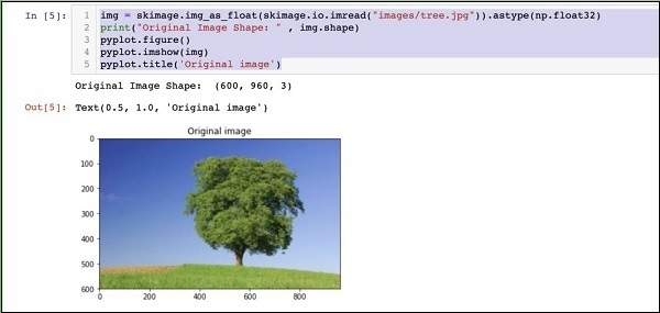
Note that size of the original image is 600 x 960. We need to resize this to our specification of 227 x 227. Calling our earlier-defined resizefunction does this job.

img = resize(img, INPUT_IMAGE_SIZE, INPUT_IMAGE_SIZE)
print("Image Shape after resizing: " , img.shape)
pyplot.figure()
pyplot.imshow(img)
pyplot.title('Resized image')

The output is as given below −

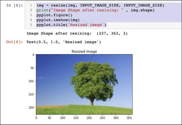
Note that now the image size is 227 x 363. We need to crop this to 227 x 227 for the final feed to our algorithm. We call the previously-defined crop function for this purpose.

img = crop_image(img, INPUT_IMAGE_SIZE, INPUT_IMAGE_SIZE)
print("Image Shape after cropping: " , img.shape)
pyplot.figure()
pyplot.imshow(img)
pyplot.title('Center Cropped')

Below mentioned is the output of the code −

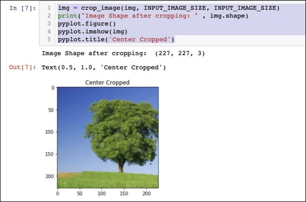
At this point, the image is of size 227 x 227 and is ready for further processing. We now swap the image axes to extract the three colours into three different zones.

img = img.swapaxes(1, 2).swapaxes(0, 1)
print("CHW Image Shape: " , img.shape)

Given below is the output −

CHW Image Shape: (3, 227, 227)

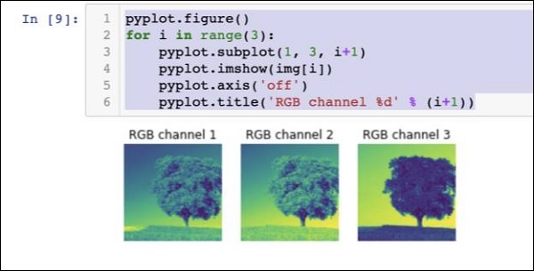
Note that the last axis has now become the first dimension in the array. We will now plot the three channels using the following code −

pyplot.figure()
for i in range(3):
   pyplot.subplot(1, 3, i+1)
   pyplot.imshow(img[i])
   pyplot.axis('off')
   pyplot.title('RGB channel %d' % (i+1))

The output is stated below −

Finally, we do some additional processing on the image such as converting Red Green Blue to Blue Green Red (RGB to BGR), removing mean for better results and adding batch size axis using the following three lines of code −

# convert RGB --> BGR
img = img[(2, 1, 0), :, :]
# remove mean
img = img * 255 - mean
# add batch size axis
img = img[np.newaxis, :, :, :].astype(np.float32)

At this point, your image is in NCHW format and is ready for feeding into our network. Next, we will load our pre-trained model files and feed the above image into it for prediction.

Predicting Objects in Processed Image

We first setup the paths for the init and predict networks defined in the pre-trained models of Caffe.

Setting Model File Paths

Remember from our earlier discussion, all the pre-trained models are installed in the models folder. We set up the path to this folder as follows −

CAFFE_MODELS = os.path.expanduser("/anaconda3/lib/python3.7/site-packages/caffe2/python/models")

We set up the path to the init_net protobuf file of the squeezenet model as follows −

INIT_NET = os.path.join(CAFFE_MODELS, 'squeezenet', 'init_net.pb')

Likewise, we set up the path to the predict_net protobuf as follows −

PREDICT_NET = os.path.join(CAFFE_MODELS, 'squeezenet', 'predict_net.pb')

We print the two paths for diagnosis purpose −

print(INIT_NET)
print(PREDICT_NET)

The above code along with the output is given here for your quick reference −

CAFFE_MODELS = os.path.expanduser("/anaconda3/lib/python3.7/site-packages/caffe2/python/models")
INIT_NET = os.path.join(CAFFE_MODELS, 'squeezenet', 'init_net.pb')
PREDICT_NET = os.path.join(CAFFE_MODELS, 'squeezenet', 'predict_net.pb')
print(INIT_NET)
print(PREDICT_NET)

The output is mentioned below −

/anaconda3/lib/python3.7/site-packages/caffe2/python/models/squeezenet/init_net.pb
/anaconda3/lib/python3.7/site-packages/caffe2/python/models/squeezenet/predict_net.pb

Next, we will create a predictor.

Creating Predictor

We read the model files using the following two statements −

with open(INIT_NET, "rb") as f:
   init_net = f.read()
with open(PREDICT_NET, "rb") as f:
   predict_net = f.read()

The predictor is created by passing pointers to the two files as parameters to the Predictor function.

p = workspace.Predictor(init_net, predict_net)

The p object is the predictor, which is used for predicting the objects in any given image. Note that each input image must be in NCHW format as what we have done earlier to our tree.jpg file.

Predicting Objects

To predict the objects in a given image is trivial - just executing a single line of command. We call run method on the predictor object for an object detection in a given image.

results = p.run({'data': img})

The prediction results are now available in the results object, which we convert to an array for our readability.

results = np.asarray(results)

Print the dimensions of the array for your understanding using the following statement −

print("results shape: ", results.shape)

The output is as shown below −

results shape: (1, 1, 1000, 1, 1)

We will now remove the unnecessary axis −

preds = np.squeeze(results)

The topmost predication can now be retrieved by taking the max value in the preds array.

curr_pred, curr_conf = max(enumerate(preds), key=operator.itemgetter(1))
print("Prediction: ", curr_pred)
print("Confidence: ", curr_conf)

The output is as follows −

Prediction: 984
Confidence: 0.89235985

As you see the model has predicted an object with an index value 984 with 89% confidence. The index of 984 does not make much sense to us in understanding what kind of object is detected. We need to get the stringified name for the object using its index value. The kind of objects that the model recognizes along with their corresponding index values are available on a github repository.

Now, we will see how to retrieve the name for our object having index value of 984.

Stringifying Result

We create a URL object to the github repository as follows −

codes = "https://gist.githubusercontent.com/aaronmarkham/cd3a6b6ac0
71eca6f7b4a6e40e6038aa/raw/9edb4038a37da6b5a44c3b5bc52e448ff09bfe5b/alexnet_codes"

We read the contents of the URL −

response = urllib2.urlopen(codes)

The response will contain a list of all codes and its descriptions. Few lines of the response are shown below for your understanding of what it contains −

5: 'electric ray, crampfish, numbfish, torpedo',
6: 'stingray',
7: 'cock',
8: 'hen',
9: 'ostrich, Struthio camelus',
10: 'brambling, Fringilla montifringilla',

We now iterate the entire array to locate our desired code of 984 using a for loop as follows −

for line in response:
   mystring = line.decode('ascii')
   code, result = mystring.partition(":")[::2]
   code = code.strip()
   result = result.replace("'", "")
   if (code == str(curr_pred)):
      name = result.split(",")[0][1:]
      print("Model predicts", name, "with", curr_conf, "confidence")

When you run the code, you will see the following output −

Model predicts rapeseed with 0.89235985 confidence

You may now try the model on another image.

Predicting a Different Image

To predict another image, simply copy the image file into the images folder of your project directory. This is the directory in which our earlier tree.jpg file is stored. Change the name of the image file in the code. Only one change is required as shown below

img = skimage.img_as_float(skimage.io.imread("images/pretzel.jpg")).astype(np.float32)

The original picture and the prediction result are shown below −

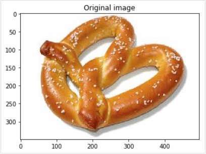
The output is mentioned below −

Model predicts pretzel with 0.99999976 confidence

As you see the pre-trained model is able to detect objects in a given image with a great amount of accuracy.

Full Source

The full source for the above code that uses a pre-trained model for object detection in a given image is mentioned here for your quick reference −

def crop_image(img,cropx,cropy):
   y,x,c = img.shape
   startx = x//2-(cropx//2)
   starty = y//2-(cropy//2)
   return img[starty:starty+cropy,startx:startx+cropx]
img = skimage.img_as_float(skimage.io.imread("images/pretzel.jpg")).astype(np.float32)
print("Original Image Shape: " , img.shape)
pyplot.figure()
pyplot.imshow(img)
pyplot.title('Original image')
img = resize(img, INPUT_IMAGE_SIZE, INPUT_IMAGE_SIZE)
print("Image Shape after resizing: " , img.shape)
pyplot.figure()
pyplot.imshow(img)
pyplot.title('Resized image')
img = crop_image(img, INPUT_IMAGE_SIZE, INPUT_IMAGE_SIZE)
print("Image Shape after cropping: " , img.shape)
pyplot.figure()
pyplot.imshow(img)
pyplot.title('Center Cropped')
img = img.swapaxes(1, 2).swapaxes(0, 1)
print("CHW Image Shape: " , img.shape)
pyplot.figure()
for i in range(3):
pyplot.subplot(1, 3, i+1)
pyplot.imshow(img[i])
pyplot.axis('off')
pyplot.title('RGB channel %d' % (i+1))
# convert RGB --> BGR
img = img[(2, 1, 0), :, :]
# remove mean
img = img * 255 - mean
# add batch size axis
img = img[np.newaxis, :, :, :].astype(np.float32)
CAFFE_MODELS = os.path.expanduser("/anaconda3/lib/python3.7/site-packages/caffe2/python/models")
INIT_NET = os.path.join(CAFFE_MODELS, 'squeezenet', 'init_net.pb')
PREDICT_NET = os.path.join(CAFFE_MODELS, 'squeezenet', 'predict_net.pb')
print(INIT_NET)
print(PREDICT_NET)
with open(INIT_NET, "rb") as f:
   init_net = f.read()
with open(PREDICT_NET, "rb") as f:
   predict_net = f.read()
p = workspace.Predictor(init_net, predict_net)
results = p.run({'data': img})
results = np.asarray(results)
print("results shape: ", results.shape)
preds = np.squeeze(results)
curr_pred, curr_conf = max(enumerate(preds), key=operator.itemgetter(1))
print("Prediction: ", curr_pred)
print("Confidence: ", curr_conf)
codes = "https://gist.githubusercontent.com/aaronmarkham/cd3a6b6ac071eca6f7b4a6e40e6038aa/raw/9edb4038a37da6b5a44c3b5bc52e448ff09bfe5b/alexnet_codes"
response = urllib2.urlopen(codes)
for line in response:
   mystring = line.decode('ascii')
   code, result = mystring.partition(":")[::2]
   code = code.strip()
   result = result.replace("'", "")
   if (code == str(curr_pred)):
      name = result.split(",")[0][1:]
      print("Model predicts", name, "with", curr_conf, "confidence")

By this time, you know how to use a pre-trained model for doing the predictions on your dataset.

What’s next is to learn how to define your neural network (NN) architectures in Caffe2 and train them on your dataset. We will now learn how to create a trivial single layer NN.