Caffe2 - Creating Your Own Network

---

---

In this lesson, you will learn to define a single layer neural network (NN) in Caffe2 and run it on a randomly generated dataset. We will write code to graphically depict the network architecture, print input, output, weights, and bias values. To understand this lesson, you must be familiar with neural network architectures, its terms and mathematics used in them.

Network Architecture

Let us consider that we want to build a single layer NN as shown in the figure below −

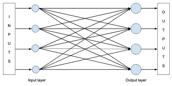
Mathematically, this network is represented by the following Python code −

Y = X * W^T + b

Where X, W, b are tensors and Y is the output. We will fill all three tensors with some random data, run the network and examine the Y output. To define the network and tensors, Caffe2 provides several Operator functions.

Caffe2 Operators

In Caffe2, Operator is the basic unit of computation. The Caffe2 Operator is represented as follows.

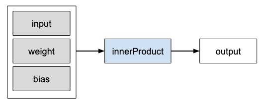
Caffe2 provides an exhaustive list of operators. For the network that we are designing currently, we will use the operator called FC, which computes the result of passing an input vector X into a fully connected network with a two-dimensional weight matrix W and a single-dimensional bias vector b. In other words, it computes the following mathematical equation

Y = X * W^T + b

Where X has dimensions (M x k), W has dimensions (n x k) and b is (1 x n). The output Y will be of dimension (M x n), where M is the batch size.

For the vectors X and W, we will use the GaussianFill operator to create some random data. For generating bias values b, we will use ConstantFill operator.

We will now proceed to define our network.

Creating Network

First of all, import the required packages −

from caffe2.python import core, workspace

Next, define the network by calling core.Net as follows −

net = core.Net("SingleLayerFC")

The name of the network is specified as SingleLayerFC. At this point, the network object called net is created. It does not contain any layers so far.

Creating Tensors

We will now create the three vectors required by our network. First, we will create X tensor by calling GaussianFill operator as follows −

X = net.GaussianFill([], ["X"], mean=0.0, std=1.0, shape=[2, 3], run_once=0)

The X vector has dimensions 2 x 3 with the mean data value of 0,0 and standard deviation of 1.0.

Likewise, we create W tensor as follows −

W = net.GaussianFill([], ["W"], mean=0.0, std=1.0, shape=[5, 3], run_once=0)

The W vector is of size 5 x 3.

Finally, we create bias b matrix of size 5.

b = net.ConstantFill([], ["b"], shape=[5,], value=1.0, run_once=0)

Now, comes the most important part of the code and that is defining the network itself.

Defining Network

We define the network in the following Python statement −

Y = X.FC([W, b], ["Y"])

We call FC operator on the input data X. The weights are specified in W and bias in b. The output is Y. Alternatively, you may create the network using the following Python statement, which is more verbose.

Y = net.FC([X, W, b], ["Y"])

At this point, the network is simply created. Until we run the network at least once, it will not contain any data. Before running the network, we will examine its architecture.

Printing Network Architecture

Caffe2 defines the network architecture in a JSON file, which can be examined by calling the Proto method on the created net object.

print (net.Proto())

This produces the following output −

name: "SingleLayerFC"
op {
   output: "X"
   name: ""
   type: "GaussianFill"
   arg {
      name: "mean"
      f: 0.0
   }
   arg {
      name: "std"
      f: 1.0
   }
   arg {
      name: "shape"
      ints: 2
      ints: 3
   }
   arg {
      name: "run_once"
      i: 0
   }
}
op {
   output: "W"
   name: ""
   type: "GaussianFill"
   arg {
      name: "mean"
      f: 0.0
   }
   arg {
      name: "std"
      f: 1.0
   }
   arg {
      name: "shape"
      ints: 5
      ints: 3
   }
   arg {
      name: "run_once"
      i: 0
   }
}
op {
   output: "b"
   name: ""
   type: "ConstantFill"
   arg {
      name: "shape"
      ints: 5
   }
   arg {
      name: "value"
      f: 1.0
   }
   arg {
      name: "run_once"
      i: 0
   }
}
op {
   input: "X"
   input: "W"
   input: "b"
   output: "Y"
   name: ""
   type: "FC"
}

As you can see in the above listing, it first defines the operators X, W and b. Let us examine the definition of W as an example. The type of W is specified as GausianFill. The mean is defined as float 0.0, the standard deviation is defined as float 1.0, and the shape is 5 x 3.

op {
   output: "W"
   name: "" type: "GaussianFill"
   arg {
      name: "mean" 
	   f: 0.0
   }
   arg { 
      name: "std" 
      f: 1.0
   }
   arg { 
      name: "shape" 
      ints: 5 
      ints: 3
   }
   ...
}

Examine the definitions of X and b for your own understanding. Finally, let us look at the definition of our single layer network, which is reproduced here

op {
   input: "X"
   input: "W"
   input: "b"
   output: "Y"
   name: ""
   type: "FC"
}

Here, the network type is FC (Fully Connected) with X, W, b as inputs and Y is the output. This network definition is too verbose and for large networks, it will become tedious to examine its contents. Fortunately, Caffe2 provides a graphical representation for the created networks.

Network Graphical Representation

To get the graphical representation of the network, run the following code snippet, which is essentially only two lines of Python code.

from caffe2.python import net_drawer
from IPython import display
graph = net_drawer.GetPydotGraph(net, rankdir="LR")
display.Image(graph.create_png(), width=800)

When you run the code, you will see the following output −

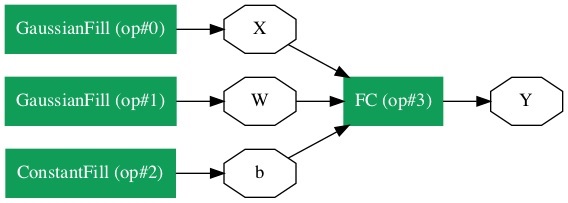
For large networks, the graphical representation becomes extremely useful in visualizing and debugging network definition errors.

Finally, it is now time to run the network.

Running Network

You run the network by calling the RunNetOnce method on the workspace object −

workspace.RunNetOnce(net)

After the network is run once, all our data that is generated at random would be created, fed into the network and the output will be created. The tensors which are created after running the network are called blobs in Caffe2. The workspace consists of the blobs you create and store in memory. This is quite similar to Matlab.

After running the network, you can examine the blobs that the workspace contains using the following print command

print("Blobs in the workspace: {}".format(workspace.Blobs()))

You will see the following output −

Blobs in the workspace: ['W', 'X', 'Y', 'b']

Note that the workspace consists of three input blobs − X, W and b. It also contains the output blob called Y. Let us now examine the contents of these blobs.

for name in workspace.Blobs():
   print("{}:\n{}".format(name, workspace.FetchBlob(name)))

You will see the following output −

W:
[[ 1.0426593 0.15479846 0.25635982]
[-2.2461145 1.4581774 0.16827184]
[-0.12009818 0.30771437 0.00791338]
[ 1.2274994 -0.903331 -0.68799865]
[ 0.30834186 -0.53060573 0.88776857]]
X:
[[ 1.6588869e+00 1.5279824e+00 1.1889904e+00]
[ 6.7048723e-01 -9.7490678e-04 2.5114202e-01]]
Y:
[[ 3.2709925 -0.297907 1.2803618 0.837985 1.7562964]
[ 1.7633215 -0.4651525 0.9211631 1.6511179 1.4302125]]
b:
[1. 1. 1. 1. 1.]

Note that the data on your machine or as a matter of fact on every run of the network would be different as all inputs are created at random. You have now successfully defined a network and run it on your computer.