AI with Python – Analyzing Time Series Data

---

---

Predicting the next in a given input sequence is another important concept in machine learning. This chapter gives you a detailed explanation about analyzing time series data.

Introduction

Time series data means the data that is in a series of particular time intervals. If we want to build sequence prediction in machine learning, then we have to deal with sequential data and time. Series data is an abstract of sequential data. Ordering of data is an important feature of sequential data.

Basic Concept of Sequence Analysis or Time Series Analysis

Sequence analysis or time series analysis is to predict the next in a given input sequence based on the previously observed. The prediction can be of anything that may come next: a symbol, a number, next day weather, next term in speech etc. Sequence analysis can be very handy in applications such as stock market analysis, weather forecasting, and product recommendations.

Example

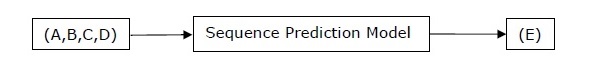
Consider the following example to understand sequence prediction. Here A,B,C,D are the given values and you have to predict the value E using a Sequence Prediction Model.

Installing Useful Packages

For time series data analysis using Python, we need to install the following packages −

Pandas

Pandas is an open source BSD-licensed library which provides high-performance, ease of data structure usage and data analysis tools for Python. You can install Pandas with the help of the following command −

pip install pandas

If you are using Anaconda and want to install by using the conda package manager, then you can use the following command −

conda install -c anaconda pandas

hmmlearn

It is an open source BSD-licensed library which consists of simple algorithms and models to learn Hidden Markov Models(HMM) in Python. You can install it with the help of the following command −

pip install hmmlearn

If you are using Anaconda and want to install by using the conda package manager, then you can use the following command −

conda install -c omnia hmmlearn

PyStruct

It is a structured learning and prediction library. Learning algorithms implemented in PyStruct have names such as conditional random fields(CRF), Maximum-Margin Markov Random Networks (M3N) or structural support vector machines. You can install it with the help of the following command −

pip install pystruct

CVXOPT

It is used for convex optimization based on Python programming language. It is also a free software package. You can install it with the help of following command −

pip install cvxopt

If you are using Anaconda and want to install by using the conda package manager, then you can use the following command −

conda install -c anaconda cvdoxt

Pandas: Handling, Slicing and Extracting Statistic from Time Series Data

Pandas is a very useful tool if you have to work with time series data. With the help of Pandas, you can perform the following −

• Create a range of dates by using the pd.date_range package

• Index pandas with dates by using the pd.Series package

• Perform re-sampling by using the ts.resample package

• Change the frequency

Example

The following example shows you handling and slicing the time series data by using Pandas. Note that here we are using the Monthly Arctic Oscillation data, which can be downloaded from monthly.ao.index.b50.current.ascii and can be converted to text format for our use.

Handling time series data

For handling time series data, you will have to perform the following steps −

The first step involves importing the following packages −

import numpy as np
import matplotlib.pyplot as plt
import pandas as pd

Next, define a function which will read the data from the input file, as shown in the code given below −

def read_data(input_file):
   input_data = np.loadtxt(input_file, delimiter = None)

Now, convert this data to time series. For this, create the range of dates of our time series. In this example, we keep one month as frequency of data. Our file is having the data which starts from January 1950.

dates = pd.date_range('1950-01', periods = input_data.shape[0], freq = 'M')

In this step, we create the time series data with the help of Pandas Series, as shown below −

output = pd.Series(input_data[:, index], index = dates)	
return output
	
if __name__=='__main__':

Enter the path of the input file as shown here −

input_file = "/Users/admin/AO.txt"

Now, convert the column to timeseries format, as shown here −

timeseries = read_data(input_file)

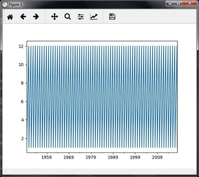
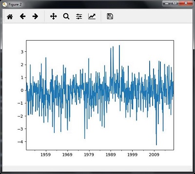
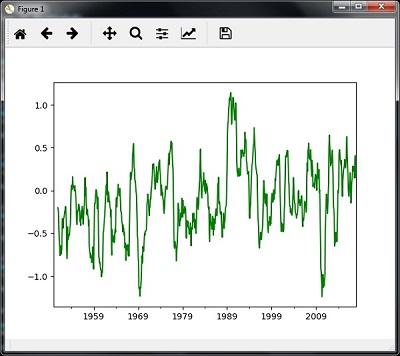
Finally, plot and visualize the data, using the commands shown −

plt.figure()
timeseries.plot()
plt.show()

You will observe the plots as shown in the following images −

Slicing time series data

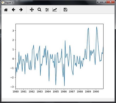
Slicing involves retrieving only some part of the time series data. As a part of the example, we are slicing the data only from 1980 to 1990. Observe the following code that performs this task −

timeseries['1980':'1990'].plot()
   <matplotlib.axes._subplots.AxesSubplot at 0xa0e4b00>

plt.show()

When you run the code for slicing the time series data, you can observe the following graph as shown in the image here −

Extracting Statistic from Time Series Data

You will have to extract some statistics from a given data, in cases where you need to draw some important conclusion. Mean, variance, correlation, maximum value, and minimum value are some of such statistics. You can use the following code if you want to extract such statistics from a given time series data −

Mean

You can use the mean() function, for finding the mean, as shown here −

timeseries.mean()

Then the output that you will observe for the example discussed is −

-0.11143128165238671

Maximum

You can use the max() function, for finding maximum, as shown here −

timeseries.max()

Then the output that you will observe for the example discussed is −

3.4952999999999999

Minimum

You can use the min() function, for finding minimum, as shown here −

timeseries.min()

Then the output that you will observe for the example discussed is −

-4.2656999999999998

Getting everything at once

If you want to calculate all statistics at a time, you can use the describe() function as shown here −

timeseries.describe()

Then the output that you will observe for the example discussed is −

count   817.000000
mean     -0.111431
std       1.003151
min      -4.265700
25%      -0.649430
50%      -0.042744
75%       0.475720
max       3.495300
dtype: float64

Re-sampling

You can resample the data to a different time frequency. The two parameters for performing re-sampling are −

• Time period
• Method

Re-sampling with mean()

You can use the following code to resample the data with the mean()method, which is the default method −

timeseries_mm = timeseries.resample("A").mean()
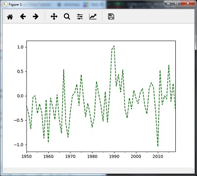
timeseries_mm.plot(style = 'g--')
plt.show()

Then, you can observe the following graph as the output of resampling using mean() −

Re-sampling with median()

You can use the following code to resample the data using the median()method −

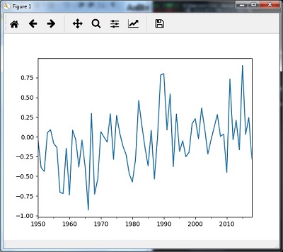
timeseries_mm = timeseries.resample("A").median()
timeseries_mm.plot()
plt.show()

Then, you can observe the following graph as the output of re-sampling with median() −

Rolling Mean

You can use the following code to calculate the rolling (moving) mean −

timeseries.rolling(window = 12, center = False).mean().plot(style = '-g')
plt.show()

Then, you can observe the following graph as the output of the rolling (moving) mean −

Analyzing Sequential Data by Hidden Markov Model (HMM)

HMM is a statistic model which is widely used for data having continuation and extensibility such as time series stock market analysis, health checkup, and speech recognition. This section deals in detail with analyzing sequential data using Hidden Markov Model (HMM).

Hidden Markov Model (HMM)

HMM is a stochastic model which is built upon the concept of Markov chain based on the assumption that probability of future stats depends only on the current process state rather any state that preceded it. For example, when tossing a coin, we cannot say that the result of the fifth toss will be a head. This is because a coin does not have any memory and the next result does not depend on the previous result.

Mathematically, HMM consists of the following variables −

States (S)

It is a set of hidden or latent states present in a HMM. It is denoted by S.

Output symbols (O)

It is a set of possible output symbols present in a HMM. It is denoted by O.

State Transition Probability Matrix (A)

It is the probability of making transition from one state to each of the other states. It is denoted by A.

Observation Emission Probability Matrix (B)

It is the probability of emitting/observing a symbol at a particular state. It is denoted by B.

Prior Probability Matrix (Π)

It is the probability of starting at a particular state from various states of the system. It is denoted by Π.

Hence, a HMM may be defined as 𝝀 = (S,O,A,B,𝝅),

where,

• S = {s₁,s₂,…,s_N} is a set of N possible states,
• O = {o₁,o₂,…,o_M} is a set of M possible observation symbols,
• A is an N𝒙N state Transition Probability Matrix (TPM),
• B is an N𝒙M observation or Emission Probability Matrix (EPM),
• π is an N dimensional initial state probability distribution vector.

Example: Analysis of Stock Market data

In this example, we are going to analyze the data of stock market, step by step, to get an idea about how the HMM works with sequential or time series data. Please note that we are implementing this example in Python.

Import the necessary packages as shown below −

import datetime
import warnings

Now, use the stock market data from the matpotlib.finance package, as shown here −

import numpy as np
from matplotlib import cm, pyplot as plt
from matplotlib.dates import YearLocator, MonthLocator
try:
   from matplotlib.finance import quotes_historical_yahoo_och1
except ImportError:
   from matplotlib.finance import (
      quotes_historical_yahoo as quotes_historical_yahoo_och1)

from hmmlearn.hmm import GaussianHMM

Load the data from a start date and end date, i.e., between two specific dates as shown here −

start_date = datetime.date(1995, 10, 10)
end_date = datetime.date(2015, 4, 25)
quotes = quotes_historical_yahoo_och1('INTC', start_date, end_date)

In this step, we will extract the closing quotes every day. For this, use the following command −

closing_quotes = np.array([quote[2] for quote in quotes])

Now, we will extract the volume of shares traded every day. For this, use the following command −

volumes = np.array([quote[5] for quote in quotes])[1:]

Here, take the percentage difference of closing stock prices, using the code shown below −

diff_percentages = 100.0 * np.diff(closing_quotes) / closing_quotes[:-]
dates = np.array([quote[0] for quote in quotes], dtype = np.int)[1:]
training_data = np.column_stack([diff_percentages, volumes])

In this step, create and train the Gaussian HMM. For this, use the following code −

hmm = GaussianHMM(n_components = 7, covariance_type = 'diag', n_iter = 1000)
with warnings.catch_warnings():
   warnings.simplefilter('ignore')
   hmm.fit(training_data)

Now, generate data using the HMM model, using the commands shown −

num_samples = 300
samples, _ = hmm.sample(num_samples)

Finally, in this step, we plot and visualize the difference percentage and volume of shares traded as output in the form of graph.

Use the following code to plot and visualize the difference percentages −

plt.figure()
plt.title('Difference percentages')
plt.plot(np.arange(num_samples), samples[:, 0], c = 'black')

Use the following code to plot and visualize the volume of shares traded −

plt.figure()
plt.title('Volume of shares')
plt.plot(np.arange(num_samples), samples[:, 1], c = 'black')
plt.ylim(ymin = 0)
plt.show()