TensorFlow - Single Layer Perceptron

---

---

For understanding single layer perceptron, it is important to understand Artificial Neural Networks (ANN). Artificial neural networks is the information processing system the mechanism of which is inspired with the functionality of biological neural circuits. An artificial neural network possesses many processing units connected to each other. Following is the schematic representation of artificial neural network −

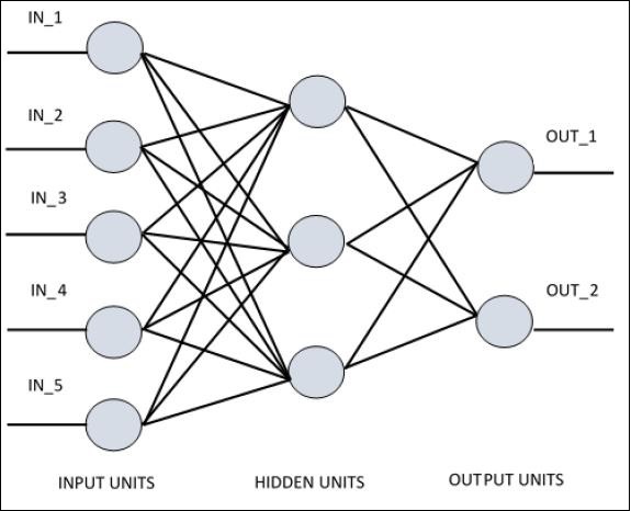
The diagram shows that the hidden units communicate with the external layer. While the input and output units communicate only through the hidden layer of the network.

The pattern of connection with nodes, the total number of layers and level of nodes between inputs and outputs with the number of neurons per layer define the architecture of a neural network.

There are two types of architecture. These types focus on the functionality artificial neural networks as follows −

• Single Layer Perceptron
• Multi-Layer Perceptron

Single Layer Perceptron

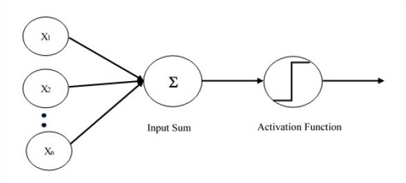
Single layer perceptron is the first proposed neural model created. The content of the local memory of the neuron consists of a vector of weights. The computation of a single layer perceptron is performed over the calculation of sum of the input vector each with the value multiplied by corresponding element of vector of the weights. The value which is displayed in the output will be the input of an activation function.

Let us focus on the implementation of single layer perceptron for an image classification problem using TensorFlow. The best example to illustrate the single layer perceptron is through representation of “Logistic Regression”.

Now, let us consider the following basic steps of training logistic regression −

• The weights are initialized with random values at the beginning of the training.

• For each element of the training set, the error is calculated with the difference between desired output and the actual output. The error calculated is used to adjust the weights.

• The process is repeated until the error made on the entire training set is not less than the specified threshold, until the maximum number of iterations is reached.

The complete code for evaluation of logistic regression is mentioned below −

# Import MINST data 
from tensorflow.examples.tutorials.mnist import input_data 
mnist = input_data.read_data_sets("/tmp/data/", one_hot = True) 

import tensorflow as tf 
import matplotlib.pyplot as plt 

# Parameters 
learning_rate = 0.01 
training_epochs = 25 
batch_size = 100 
display_step = 1 

# tf Graph Input 
x = tf.placeholder("float", [None, 784]) # mnist data image of shape 28*28 = 784 
y = tf.placeholder("float", [None, 10]) # 0-9 digits recognition => 10 classes 

# Create model 
# Set model weights 
W = tf.Variable(tf.zeros([784, 10])) 
b = tf.Variable(tf.zeros([10])) 

# Construct model 
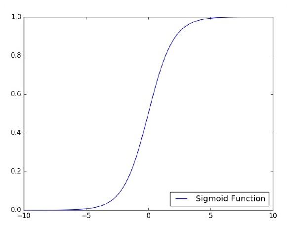
activation = tf.nn.softmax(tf.matmul(x, W) + b) # Softmax 

# Minimize error using cross entropy 
cross_entropy = y*tf.log(activation) 
cost = tf.reduce_mean\ (-tf.reduce_sum\ (cross_entropy,reduction_indices = 1)) 

optimizer = tf.train.\ GradientDescentOptimizer(learning_rate).minimize(cost) 

#Plot settings 
avg_set = [] 
epoch_set = [] 

# Initializing the variables init = tf.initialize_all_variables()
# Launch the graph 
with tf.Session() as sess:
   sess.run(init)
   
   # Training cycle
   for epoch in range(training_epochs):
      avg_cost = 0.
      total_batch = int(mnist.train.num_examples/batch_size)
      
      # Loop over all batches
      for i in range(total_batch):
         batch_xs, batch_ys = \ mnist.train.next_batch(batch_size)
         # Fit training using batch data sess.run(optimizer, \ feed_dict = {
            x: batch_xs, y: batch_ys}) 
         # Compute average loss avg_cost += sess.run(cost, \ feed_dict = {
            x: batch_xs, \ y: batch_ys})/total_batch
      # Display logs per epoch step
      if epoch % display_step == 0:
         print ("Epoch:", '%04d' % (epoch+1), "cost=", "{:.9f}".format(avg_cost))
            avg_set.append(avg_cost) epoch_set.append(epoch+1)
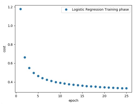
   print ("Training phase finished")
    
   plt.plot(epoch_set,avg_set, 'o', label = 'Logistic Regression Training phase') 
   plt.ylabel('cost') 
   plt.xlabel('epoch') 
   plt.legend() 
   plt.show() 
    
   # Test model 
   correct_prediction = tf.equal(tf.argmax(activation, 1), tf.argmax(y, 1)) 
   
   # Calculate accuracy 
   accuracy = tf.reduce_mean(tf.cast(correct_prediction, "float")) print 
      ("Model accuracy:", accuracy.eval({x: mnist.test.images, y: mnist.test.labels}))

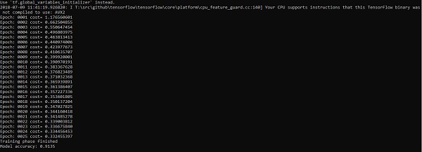
Output

The above code generates the following output −

The logistic regression is considered as a predictive analysis. Logistic regression is used to describe data and to explain the relationship between one dependent binary variable and one or more nominal or independent variables.