- Keras - Home
- Keras - Introduction
- Keras - Installation
- Keras - Backend Configuration
- Keras - Overview of Deep learning
- Keras - Deep learning
- Keras - Modules
- Keras - Layers
- Keras - Customized Layer
- Keras - Models
- Keras - Model Compilation
- Keras - Model Evaluation and Prediction
- Keras - Convolution Neural Network
- Keras - Regression Prediction using MPL
- Keras - Time Series Prediction using LSTM RNN
- Keras - Applications
- Keras - Real Time Prediction using ResNet Model
- Keras - Pre-Trained Models
- Keras Useful Resources
- Keras - Quick Guide
- Keras - Useful Resources
- Keras - Discussion
Keras - Time Series Prediction using LSTM RNN
In this chapter, let us write a simple Long Short Term Memory (LSTM) based RNN to do sequence analysis. A sequence is a set of values where each value corresponds to a particular instance of time. Let us consider a simple example of reading a sentence. Reading and understanding a sentence involves reading the word in the given order and trying to understand each word and its meaning in the given context and finally understanding the sentence in a positive or negative sentiment.
Here, the words are considered as values, and first value corresponds to first word, second value corresponds to second word, etc., and the order will be strictly maintained. Sequence Analysis is used frequently in natural language processing to find the sentiment analysis of the given text.
Let us create a LSTM model to analyze the IMDB movie reviews and find its positive/negative sentiment.
The model for the sequence analysis can be represented as below −
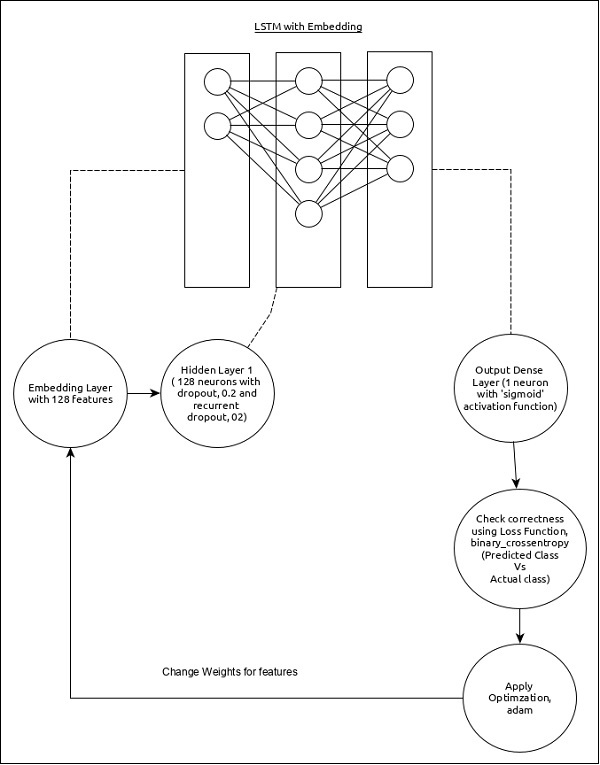
The core features of the model are as follows −
Input layer using Embedding layer with 128 features.
First layer, Dense consists of 128 units with normal dropout and recurrent dropout set to 0.2.
Output layer, Dense consists of 1 unit and sigmoid activation function.
Use binary_crossentropy as loss function.
Use adam as Optimizer.
Use accuracy as metrics.
Use 32 as batch size.
Use 15 as epochs.
Use 80 as the maximum length of the word.
Use 2000 as the maximum number of word in a given sentence.
Step 1: Import the modules
Let us import the necessary modules.
from keras.preprocessing import sequence
from keras.models import Sequential
from keras.layers import Dense, Embedding
from keras.layers import LSTM
from keras.datasets import imdb
Step 2: Load data
Let us import the imdb dataset.
(x_train, y_train), (x_test, y_test) = imdb.load_data(num_words = 2000)
Here,
imdb is a dataset provided by Keras. It represents a collection of movies and its reviews.
num_words represent the maximum number of words in the review.
Step 3: Process the data
Let us change the dataset according to our model, so that it can be fed into our model. The data can be changed using the below code −
x_train = sequence.pad_sequences(x_train, maxlen=80)
x_test = sequence.pad_sequences(x_test, maxlen=80)
Here,
sequence.pad_sequences convert the list of input data with shape, (data) into 2D NumPy array of shape (data, timesteps). Basically, it adds timesteps concept into the given data. It generates the timesteps of length, maxlen.
Step 4: Create the model
Let us create the actual model.
model = Sequential()
model.add(Embedding(2000, 128))
model.add(LSTM(128, dropout = 0.2, recurrent_dropout = 0.2))
model.add(Dense(1, activation = 'sigmoid'))
Here,
We have used Embedding layer as input layer and then added the LSTM layer. Finally, a Dense layer is used as output layer.
Step 5: Compile the model
Let us compile the model using selected loss function, optimizer and metrics.
model.compile(loss = 'binary_crossentropy',
   optimizer = 'adam', metrics = ['accuracy'])
Step 6: Train the model
LLet us train the model using fit() method.
model.fit(
   x_train, y_train,
   batch_size = 32,
   epochs = 15,
   validation_data = (x_test, y_test)
)
Executing the application will output the below information −
Epoch 1/15 2019-09-24 01:19:01.151247: I
tensorflow/core/platform/cpu_feature_guard.cc:142]
Your CPU supports instructions that this
TensorFlow binary was not co mpiled to use: AVX2
25000/25000 [==============================] - 101s 4ms/step - loss: 0.4707
- acc: 0.7716 - val_loss: 0.3769 - val_acc: 0.8349 Epoch 2/15
25000/25000 [==============================] - 95s 4ms/step - loss: 0.3058
- acc: 0.8756 - val_loss: 0.3763 - val_acc: 0.8350 Epoch 3/15
25000/25000 [==============================] - 91s 4ms/step - loss: 0.2100
- acc: 0.9178 - val_loss: 0.5065 - val_acc: 0.8110 Epoch 4/15
25000/25000 [==============================] - 90s 4ms/step - loss: 0.1394
- acc: 0.9495 - val_loss: 0.6046 - val_acc: 0.8146 Epoch 5/15
25000/25000 [==============================] - 90s 4ms/step - loss: 0.0973
- acc: 0.9652 - val_loss: 0.5969 - val_acc: 0.8147 Epoch 6/15
25000/25000 [==============================] - 98s 4ms/step - loss: 0.0759
- acc: 0.9730 - val_loss: 0.6368 - val_acc: 0.8208 Epoch 7/15
25000/25000 [==============================] - 95s 4ms/step - loss: 0.0578
- acc: 0.9811 - val_loss: 0.6657 - val_acc: 0.8184 Epoch 8/15
25000/25000 [==============================] - 97s 4ms/step - loss: 0.0448
- acc: 0.9850 - val_loss: 0.7452 - val_acc: 0.8136 Epoch 9/15
25000/25000 [==============================] - 95s 4ms/step - loss: 0.0324
- acc: 0.9894 - val_loss: 0.7616 - val_acc: 0.8162Epoch 10/15
25000/25000 [==============================] - 100s 4ms/step - loss: 0.0247
- acc: 0.9922 - val_loss: 0.9654 - val_acc: 0.8148 Epoch 11/15
25000/25000 [==============================] - 99s 4ms/step - loss: 0.0169
- acc: 0.9946 - val_loss: 1.0013 - val_acc: 0.8104 Epoch 12/15
25000/25000 [==============================] - 90s 4ms/step - loss: 0.0154
- acc: 0.9948 - val_loss: 1.0316 - val_acc: 0.8100 Epoch 13/15
25000/25000 [==============================] - 89s 4ms/step - loss: 0.0113
- acc: 0.9963 - val_loss: 1.1138 - val_acc: 0.8108 Epoch 14/15
25000/25000 [==============================] - 89s 4ms/step - loss: 0.0106
- acc: 0.9971 - val_loss: 1.0538 - val_acc: 0.8102 Epoch 15/15
25000/25000 [==============================] - 89s 4ms/step - loss: 0.0090
- acc: 0.9972 - val_loss: 1.1453 - val_acc: 0.8129
25000/25000 [==============================] - 10s 390us/step
Step 7 − Evaluate the model
Let us evaluate the model using test data.
score, acc = model.evaluate(x_test, y_test, batch_size = 32)

print('Test score:', score)
print('Test accuracy:', acc)
Executing the above code will output the below information −
Test score: 1.145306069601178
Test accuracy: 0.81292