Haskell - Quick Guide

---

---

Haskell - Overview

Haskell is a Functional Programming Language that has been specially designed to handle symbolic computation and list processing applications. Functional programming is based on mathematical functions. Besides Haskell, some of the other popular languages that follow Functional Programming paradigm include: Lisp, Python, Erlang, Racket, F#, Clojure, etc.

In conventional programing, instructions are taken as a set of declarations in a specific syntax or format, but in the case of functional programing, all the computation is considered as a combination of separate mathematical functions.

Going Functional with Haskell

Haskell is a widely used purely functional language. Here, we have listed down a few points that make this language so special over other conventional programing languages such as Java, C, C++, PHP, etc.

• Functional Language − In conventional programing language, we instruct the compiler a series of tasks which is nothing but telling your computer "what to do" and "how to do?" But in Haskell we will tell our computer "what it is?"

• Laziness − Haskell is a lazy language. By lazy, we mean that Haskell won't evaluate any expression without any reason. When the evaluation engine finds that an expression needs to be evaluated, then it creates a thunk data structure to collect all the required information for that specific evaluation and a pointer to that thunk data structure. The evaluation engine will start working only when it is required to evaluate that specific expression.

• Modularity − A Haskell application is nothing but a series of functions. We can say that a Haskell application is a collection of numerous small Haskell applications.

• Statically Typed − In conventional programing language, we need to define a series of variables along with their type. In contrast, Haskell is a type interference language. By the term, type interference language, we mean the Haskell compiler is intelligent enough to figure out the type of the variable declared, hence we need not explicitly mention the type of the variable used.

• Maintainability − Haskell applications are modular and hence, it is very easy and cost-effective to maintain them.

Functional programs are more concurrent and they follow parallelism in execution to provide more accurate and better performance. Haskell is no exception; it has been developed in a way to handle multithreading effectively.

Hello World

It is a simple example to demonstrate the dynamism of Haskell. Take a look at the following code. All that we need is just one line to print "Hello Word" on the console.

main = putStrLn "Hello World"

Once the Haskell compiler encounters the above piece of code, it promptly yields the following output −

Hello World 

We will provide plenty of examples throughout this tutorial to showcase the power and simplicity of Haskell.

Haskell - Environment Set Up

We have set up the Haskell programing environment online at − https://www.tutorialspoint.com/compile_haskell_online.php

This online editor has plenty of options to practice Haskell programing examples. Go to the terminal section of the page and type "ghci". This command automatically loads Haskell compiler and starts Haskell online. You will receive the following output after using the ghci command.

sh-4.3$ ghci
GHCi,version7.8.4:http://www.haskell.org/ghc/:?forhelp
Loading package ghc-prim...linking...done.
Loading packageinteger gmp...linking... done.
Loading package base...linking...done.
Prelude>

If you still want to use Haskell offline in your local system, then you need to download the available Haskell setup from its official webpage − https://www.haskell.org/downloads

There are three different types of installers available in the market −

• Minimal Installer − It provides GHC (The Glasgow Haskell Compiler), CABAL (Common Architecture for Building Applications and Libraries), and Stack tools.

• Stack Installer − In this installer, the GHC can be downloaded in a cross-platform of managed toll chain. It will install your application globally such that it can update its API tools whenever required. It automatically resolves all the Haskell-oriented dependencies.

• Haskell Platform − This is the best way to install Haskell because it will install the entire platform in your machine and that to from one specific location. This installer is not distributive like the above two installers.

We have seen different types of installer available in market now let us see how to use those installers in our machine. In this tutorial we are going to use Haskell platform installer to install Haskell compiler in our system.

Environment Set Up in Windows

To set up Haskell environment on your Windows computer, go to their official website https://www.haskell.org/platform/windows.html and download the Installer according to your customizable architecture.

Check out your system’s architecture and download the corresponding setup file and run it. It will install like any other Windows application. You may need to update the CABAL configuration of your system.

Environment Set Up in MAC

To set up Haskell environment on your MAC system, go to their official website https://www.haskell.org/platform/mac.html and download the Mac installer.

Environment Set Up in Linux

Installing Haskell on a Linux-based system requires to run some command which is not that much easy like MAC and Windows. Yes, it is tiresome but it is reliable.

You can follow the steps given below to install Haskell on your Linux system −

Step 1 − To set up Haskell environment on your Linux system, go to the official website https://www.haskell.org/platform/linux.html and choose your distribution. You will find the following screen on your browser.

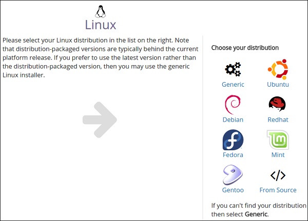
Step 2 − Select your Distribution. In our case, we are using Ubuntu. After selecting this option, you will get the following page on your screen with the command to install the Haskell in our local system.

Step 3 − Open a terminal by pressing Ctrl + Alt + T. Run the command "$ sudo apt-get install haskell-platform" and press Enter. It will automatically start downloading Haskell on your system after authenticating you with the root password. After installing, you will receive a confirmation message.

Step 4 − Go to your terminal again and run the GHCI command. Once you get the Prelude prompt, you are ready to use Haskell on your local system.

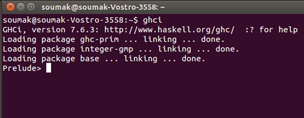
To exit from the GHCI prolog, you can use the command ":quit exit".

Haskell - Basic Data Models

Haskell is a purely functional programing language, hence it is much more interactive and intelligent than other programming languages. In this chapter, we will learn about basic data models of Haskell which are actually predefined or somehow intelligently decoded into the computer memory.

Throughout this tutorial, we will use the Haskell online platform available on our website (https://www.tutorialspoint.com/codingground.htm).

Numbers

Haskell is intelligent enough to decode some number as a number. Therefore, you need not mention its type externally as we usually do in case of other programing languages. As per example go to your prelude command prompt and just run "2+2" and hit enter.

sh-4.3$ ghci 
GHCi, version 7.6.3: http://www.haskell.org/ghc/  :? for help 
Loading package ghc-prim ... linking ... done. 
Loading package integer-gmp ... linking ... done. 
Loading package base ... linking ... done. 
Prelude> 2+2

You will receive the following output as a result.

4

In the above code, we just passed two numbers as arguments to the GHCI compiler without predefining their type, but compiler could easily decode these two entries as numbers.

Now, let us try a little more complex mathematical calculation and see whether our intelligent compiler give us the correct output or not. Try with "15+(5*5)-40"

Prelude> 15+(5*5)-40 

The above expression yields "0" as per the expected output.

0

Characters

Like numbers, Haskell can intelligently identify a character given in as an input to it. Go to your Haskell command prompt and type any character with double or single quotation.

Let us provide following line as input and check its output.

Prelude> :t "a" 

It will produce the following output −

"a" :: [Char] 

Remember you use (:t) while supplying the input. In the above example, (:t) is to include the specific type related to the inputs. We will learn more about this type in the upcoming chapters.

Take a look at the following example where we are passing some invalid input as a char which in turn leads to an error.

Prelude> :t a 
<interactive>:1:1: Not in scope: 'a'  

Prelude> a 
<interactive>:4:1: Not in scope: 'a' 

By the error message "<interactive>:4:1: Not in scope: `a'" the Haskell compiler is warning us that it is not able to recognize your input. Haskell is a type of language where everything is represented using a number.

Haskell follows conventional ASCII encoding style. Let us take a look at the following example to understand more −

Prelude> '\97' 
'a'  
Prelude> '\67' 
'C' 

Look how your input gets decoded into ASCII format.

String

A string is nothing but a collection of characters. There is no specific syntax for using string, but Haskell follows the conventional style of representing a string with double quotation.

Take a look at the following example where we are passing the string “Tutorialspoint.com”.

Prelude> :t "tutorialspoint.com" 

It will produce the following output on screen −

"tutorialspoint.com" :: [Char] 

See how the entire string has been decoded as an array of Char only. Let us move to the other data type and its syntax. Once we start our actual practice, we will be habituated with all the data type and its use.

Boolean

Boolean data type is also pretty much straightforward like other data type. Look at the following example where we will use different Boolean operations using some Boolean inputs such as "True" or "False".

Prelude> True && True 
True  
Prelude> True && False 
False   
Prelude> True || True 
True  
Prelude> True || False 
True

In the above example, we need not mention that "True" and "False" are the Boolean values. Haskell itself can decode it and do the respective operations. Let us modify our inputs with "true" or "false".

Prelude> true 

It will produce the following output −

<interactive>:9:1: Not in scope: 'true' 

In the above example, Haskell could not differentiate between "true" and a number value, hence our input "true" is not a number. Hence, the Haskell compiler throws an error stating that our input is not its scope.

List and List Comprehension

Like other data types, List is also a very useful data type used in Haskell. As per example, [a,b,c] is a list of characters, hence, by definition, List is a collection of same data type separated by comma.

Like other data types, you need not declare a List as a List. Haskell is intelligent enough to decode your input by looking at the syntax used in the expression.

Take a look at the following example which shows how Haskell treats a List.

Prelude> [1,2,3,4,5] 

It will produce the following output −

[1,2,3,4,5] 

Lists in Haskell are homogeneous in nature, which means they won’t allow you to declare a list of different kind of data type. Any list like [1,2,3,4,5,a,b,c,d,e,f] will produce an error.

Prelude> [1,2,3,4,5,a,b,c,d,e,f] 

This code will produce the following error −

<interactive>:17:12: Not in scope: 'a' 
<interactive>:17:14: Not in scope: 'b' 
<interactive>:17:16: Not in scope: 'c' 
<interactive>:17:18: Not in scope: 'd' 
<interactive>:17:20: Not in scope: 'e' 
<interactive>:17:22: Not in scope: 'f'

List Comprehension

List comprehension is the process of generating a list using mathematical expression. Look at the following example where we are generating a list using mathematical expression in the format of [output | range ,condition].

Prelude> [x*2| x<-[1..10]] 
[2,4,6,8,10,12,14,16,18,20]  
Prelude> [x*2| x<-[1..5]] 
[2,4,6,8,10]  
Prelude> [x| x<-[1..5]] 
[1,2,3,4,5]

This method of creating one List using mathematical expression is called as List Comprehension.

Tuple

Haskell provides another way to declare multiple values in a single data type. It is known as Tuple. A Tuple can be considered as a List, however there are some technical differences in between a Tuple and a List.

A Tuple is an immutable data type, as we cannot modify the number of elements at runtime, whereas a List is a mutable data type.

On the other hand, List is a homogeneous data type, but Tuple is heterogeneous in nature, because a Tuple may contain different type of data inside it.

Tuples are represented by single parenthesis. Take a look at the following example to see how Haskell treats a Tuple.

Prelude> (1,1,'a') 

It will produce the following output −

(1,1,'a') 

In the above example, we have used one Tuple with two number type variables, and a char type variable.

Haskell - Basic Operators

In this chapter, we will learn about different operators used in Haskell. Like other programming languages, Haskell intelligently handles some basic operations like addition, subtraction, multiplication, etc. In the upcoming chapters, we will learn more about different operators and their use.

In this chapter, we will use different operators in Haskell using our online platform (https://www.tutorialspoint.com/codingground.htm). Remember we are using only integer type numbers because we will learn more about decimal type numbers in the subsequent chapters.

Addition Operator

As the name suggests, the addition (+) operator is used for addition function. The following sample code shows how you can add two integer numbers in Haskell −

main = do 
   let var1 = 2 
   let var2 = 3 
   putStrLn "The addition of the two numbers is:" 
   print(var1 + var2) 

In the above file, we have created two separate variables var1 and var2. At the end, we are printing the result using the addition operator. Use the compile and execute button to run your code.

This code will produce the following output on screen −

The addition of the two numbers is:
5

Subtraction Operator

As the name suggests, this operator is used for subtraction operation. The following sample code shows how you can subtract two integer numbers in Haskell −

main = do 
   let var1 = 10 
   let var2 = 6 
   putStrLn "The Subtraction of the two numbers is:" 
   print(var1 - var2)

In this example, we have created two variables var1 and var2. Thereafter, we use the subtraction (−) operator to subtract the two values.

This code will produce the following output on screen −

The Subtraction of the two numbers is:
4

Multiplication Operator

This operator is used for multiplication operations. The following code shows how to multiply two numbers in Haskell using the Multiplication Operator −

main = do 
   let var1 = 2 
   let var2 = 3 
   putStrLn "The Multiplication of the Two Numbers is:" 
   print(var1 * var2) 

This code will produce the following output, when you run it in our online platform −

The Multiplication of the Two Numbers is:
6 

Division Operator

Take a look at the following code. It shows how you can divide two numbers in Haskell −

main = do 
   let var1 = 12 
   let var2 = 3 
   putStrLn "The Division of the Two Numbers is:" 
   print(var1/var2)

It will produce the following output −

The Division of the Two Numbers is: 
4.0 

Sequence / Range Operator

Sequence or Range is a special operator in Haskell. It is denoted by "(..)". You can use this operator while declaring a list with a sequence of values.

If you want to print all the values from 1 to 10, then you can use something like "[1..10]". Similarly, if you want to generate all the alphabets from "a" to "z", then you can just type "[a..z]".

The following code shows how you can use the Sequence operator to print all the values from 1 to 10 −

main :: IO() 
main = do 
   print [1..10]

It will generate the following output −

[1,2,3,4,5,6,7,8,9,10] 

Haskell - Decision Making

Decision Making is a feature that allows the programmers to apply a condition in the code flow. The programmer can execute a set of instructions depending on a predefined condition. The following flowchart shows the decision-making structure of Haskell −

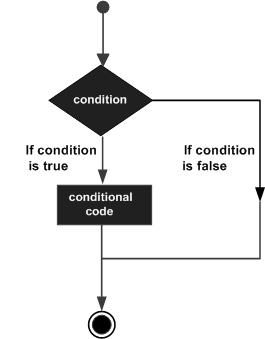
Haskell provides the following types of decision-making statements −

Haskell - Types and Type Class

Haskell is a functional language and it is strictly typed, which means the data type used in the entire application will be known to the compiler at compile time.

Inbuilt Type Class

In Haskell, every statement is considered as a mathematical expression and the category of this expression is called as a Type. You can say that "Type" is the data type of the expression used at compile time.

To learn more about the Type, we will use the ":t" command. In a generic way, Type can be considered as a value, whereas Type Class can be the considered as a set of similar kind of Types. In this chapter, we will learn about different Inbuilt Types.

Int

Int is a type class representing the Integer types data. Every whole number within the range of 2147483647 to -2147483647 comes under the Int type class. In the following example, the function fType() will behave according to its type defined.

fType :: Int -> Int -> Int 
fType x y = x*x + y*y
main = print (fType 2 4) 

Here, we have set the type of the function fType() as int. The function takes two int values and returns one int value. If you compile and execute this piece of code, then it will produce the following output −

sh-4.3$ ghc -O2 --make *.hs -o main -threaded -rtsopts 
sh-4.3$ main
20

Integer

Integer can be considered as a superset of Int. This value is not bounded by any number, hence an Integer can be of any length without any limitation. To see the basic difference between Int and Integer types, let us modify the above code as follows −

fType :: Int -> Int -> Int 
fType x y = x*x + y*y 
main = print (fType 212124454 44545454454554545445454544545)

If you compile the above piece of code, the following error message will be thrown −

main.hs:3:31: Warning:            
   Literal 44545454454554545445454544545 is out of the Int range -
   9223372036854775808..9223372036854775807 
Linking main ...

This error occurred because our function fType() expecting one Int type value, and we are passing some real big Int type value. To avoid this error, Let us modify the type "Int" with "Integer" and observe the difference.

fType :: Integer -> Integer -> Integer 
fType x y = x*x + y*y 
main = print (fType 212124454 4454545445455454545445445454544545) 

Now, it will produce the following output −

sh-4.3$ main
1984297512562793395882644631364297686099210302577374055141

Float

Take a look at the following piece of code. It shows how Float type works in Haskell −

fType :: Float -> Float -> Float 
fType x y = x*x + y*y 
main = print (fType 2.5 3.8)

The function takes two float values as the input and yields another float value as the output. When you compile and execute this code, it will produce the following output −

sh-4.3$ main
20.689999 

Double

Double is a floating point number with double precision at the end. Take a look at the following example −

fType :: Double -> Double -> Double 
fType x y = x*x + y*y 
main = print (fType 2.56 3.81)

When you execute the above piece of code, it will generate the following output −

sh-4.3$ main 
21.0697

Bool

Bool is a Boolean Type. It can be either True or False. Execute the following code to understand how the Bool type works in Haskell −

main = do  
   let x = True 
   
   if x == False 
      then putStrLn "X matches with Bool Type" 
   else putStrLn "X is not a Bool Type" 

Here, we are defining a variable "x" as a Bool and comparing it with another Boolean value to check its originality. It will produce the following output −

sh-4.3$ main
X is not a Bool Type 

Char

Char represent Characters. Anything within a single quote is considered as a Character. In the following code, we have modified our previous fType() function to accept Char value and return Char value as output.

fType :: Char-> Char 
fType x = 'K' 
main = do  
   let x = 'v' 
   print (fType x) 

The above piece of code will call fType() function with a char value of 'v' but it returns another char value, that is, 'K'. Here is its output −

sh-4.3$ main 
'K'

Note that we are not going to use these types explicitly because Haskell is intelligent enough to catch the type before it is declared. In the subsequent chapters of this tutorial, we will see how different types and Type classes make Haskell a strongly typed language.

EQ Type Class

EQ type class is an interface which provides the functionality to test the equality of an expression. Any Type class that wants to check the equality of an expression should be a part of this EQ Type Class.

All standard Type classes mentioned above is a part of this EQ class. Whenever we are checking any equality using any of the types mentioned above, we are actually making a call to EQ type class.

In the following example, we are using the EQ Type internally using the "==" or "/=" operation.

main = do 
   if 8 /= 8 
      then putStrLn "The values are Equal" 
   else putStrLn "The values are not Equal"

It will yield the following output −

sh-4.3$ main 
The values are not Equal 

Ord Type Class

Ord is another interface class which gives us the functionality of ordering. All the types that we have used so far are a part of this Ord interface. Like EQ interface, Ord interface can be called using ">", "<", "<=", ">=", "compare".

Please find below example where we used “compare ” functionality of this Type Class.

main = print (4 <= 2) 

Here, the Haskell compiler will check if 4 is less than or equal to 2. Since it is not, the code will produce the following output −

sh-4.3$ main 
False

Show

Show has a functionality to print its argument as a String. Whatever may be its argument, it always prints the result as a String. In the following example, we will print the entire list using this interface. "show" can be used to call this interface.

main = print (show [1..10]) 

It will produce the following output on the console. Here, the double quotes indicate that it is a String type value.

sh-4.3$ main 
"[1,2,3,4,5,6,7,8,9,10]" 

Read

Read interface does the same thing as Show, but it won’t print the result in String format. In the following code, we have used the read interface to read a string value and convert the same into an Int value.

main = print (readInt "12") 
readInt :: String -> Int 
readInt = read 

Here, we are passing a String variable ("12") to the readInt method which in turn returns 12 (an Int value) after conversion. Here is its output −

sh-4.3$ main 
12

Enum

Enum is another type of Type class which enables the sequential or ordered functionality in Haskell. This Type class can be accessed by commands such as Succ, Pred, Bool, Char, etc.

The following code shows how to find the successor value of 12.

main = print (succ 12) 

It will produce the following output −

sh-4.3$ main
13

Bounded

All the types having upper and lower bounds come under this Type Class. For example, Int type data has maximum bound of "9223372036854775807" and minimum bound of "-9223372036854775808".

The following code shows how Haskell determines the maximum and minimum bound of Int type.

main = do 
   print (maxBound :: Int) 
   print (minBound :: Int) 

It will produce the following output −

sh-4.3$ main
9223372036854775807
-9223372036854775808

Now, try to find the maximum and minimum bound of Char, Float, and Bool types.

Num

This type class is used for numeric operations. Types such as Int, Integer, Float, and Double come under this Type class. Take a look at the following code −

main = do 
   print(2 :: Int)  
   print(2 :: Float) 

It will produce the following output −

sh-4.3$ main
2
2.0

Integral

Integral can be considered as a sub-class of the Num Type Class. Num Type class holds all types of numbers, whereas Integral type class is used only for integral numbers. Int and Integer are the types under this Type class.

Floating

Like Integral, Floating is also a part of the Num Type class, but it only holds floating point numbers. Hence, Float and Double come under this type class.

Custom Type Class

Like any other programming language, Haskell allows developers to define user-defined types. In the following example, we will create a user-defined type and use it.

data Area = Circle Float Float Float  
surface :: Area -> Float   
surface (Circle _ _ r) = pi * r ^ 2   
main = print (surface $ Circle 10 20 10 ) 

Here, we have created a new type called Area. Next, we are using this type to calculate the area of a circle. In the above example, "surface" is a function that takes Area as an input and produces Float as the output.

Keep in mind that "data" is a keyword here and all user-defined types in Haskell always start with a capital letter.

It will produce the following output −

sh-4.3$ main
314.15927

Haskell - Functions

Functions play a major role in Haskell, as it is a functional programming language. Like other languages, Haskell does have its own functional definition and declaration.

• Function declaration consists of the function name and its argument list along with its output.

• Function definition is where you actually define a function.

Let us take small example of add function to understand this concept in detail.

add :: Integer -> Integer -> Integer   --function declaration 
add x y =  x + y                       --function definition 

main = do 
   putStrLn "The addition of the two numbers is:"  
   print(add 2 5)    --calling a function 

Here, we have declared our function in the first line and in the second line, we have written our actual function that will take two arguments and produce one integer type output.

Like most other languages, Haskell starts compiling the code from the main method. Our code will generate the following output −

The addition of the two numbers is:
7

Pattern Matching

Pattern Matching is process of matching specific type of expressions. It is nothing but a technique to simplify your code. This technique can be implemented into any type of Type class. If-Else can be used as an alternate option of pattern matching.

Pattern Matching can be considered as a variant of dynamic polymorphism where at runtime, different methods can be executed depending on their argument list.

Take a look at the following code block. Here we have used the technique of Pattern Matching to calculate the factorial of a number.

fact :: Int -> Int 
fact 0 = 1 
fact n = n * fact ( n - 1 ) 

main = do 
   putStrLn "The factorial of 5 is:" 
   print (fact 5)

We all know how to calculate the factorial of a number. The compiler will start searching for a function called "fact" with an argument. If the argument is not equal to 0, then the number will keep on calling the same function with 1 less than that of the actual argument.

When the pattern of the argument exactly matches with 0, it will call our pattern which is "fact 0 = 1". Our code will produce the following output −

The factorial of 5 is:
120

Guards

Guards is a concept that is very similar to pattern matching. In pattern matching, we usually match one or more expressions, but we use guards to test some property of an expression.

Although it is advisable to use pattern matching over guards, but from a developer’s perspective, guards is more readable and simple. For first-time users, guards can look very similar to If-Else statements, but they are functionally different.

In the following code, we have modified our factorial program by using the concept of guards.

fact :: Integer -> Integer 
fact n | n == 0 = 1 
       | n /= 0 = n * fact (n-1) 
main = do 
   putStrLn "The factorial of 5 is:"  
   print (fact 5) 

Here, we have declared two guards, separated by "|" and calling the fact function from main. Internally, the compiler will work in the same manner as in the case of pattern matching to yield the following output −

The factorial of 5 is:
120

Where Clause

Where is a keyword or inbuilt function that can be used at runtime to generate a desired output. It can be very helpful when function calculation becomes complex.

Consider a scenario where your input is a complex expression with multiple parameters. In such cases, you can break the entire expression into small parts using the "where" clause.

In the following example, we are taking a complex mathematical expression. We will show how you can find the roots of a polynomial equation [x^2 - 8x + 6] using Haskell.

roots :: (Float, Float, Float) -> (Float, Float)  
roots (a,b,c) = (x1, x2) where 
   x1 = e + sqrt d / (2 * a) 
   x2 = e - sqrt d / (2 * a) 
   d = b * b - 4 * a * c  
   e = - b / (2 * a)  
main = do 
   putStrLn "The roots of our Polynomial equation are:" 
   print (roots(1,-8,6))

Notice the complexity of our expression to calculate the roots of the given polynomial function. It is quite complex. Hence, we are breaking the expression using the where clause. The above piece of code will generate the following output −

The roots of our Polynomial equation are:
(7.1622777,0.8377223)

Recursion Function

Recursion is a situation where a function calls itself repeatedly. Haskell does not provide any facility of looping any expression for more than once. Instead, Haskell wants you to break your entire functionality into a collection of different functions and use recursion technique to implement your functionality.

Let us consider our pattern matching example again, where we have calculated the factorial of a number. Finding the factorial of a number is a classic case of using Recursion. Here, you might, "How is pattern matching any different from recursion?” The difference between these two lie in the way they are used. Pattern matching works on setting up the terminal constrain, whereas recursion is a function call.

In the following example, we have used both pattern matching and recursion to calculate the factorial of 5.

fact :: Int -> Int 
fact 0 = 1 
fact n = n * fact ( n - 1 ) 

main = do 
   putStrLn "The factorial of 5 is:" 
   print (fact 5) 

It will produce the following output −

The factorial of 5 is:
120

Higher Order Function

Till now, what we have seen is that Haskell functions take one type as input and produce another type as output, which is pretty much similar in other imperative languages. Higher Order Functions are a unique feature of Haskell where you can use a function as an input or output argument.

Although it is a virtual concept, but in real-world programs, every function that we define in Haskell use higher-order mechanism to provide output. If you get a chance to look into the library function of Haskell, then you will find that most of the library functions have been written in higher order manner.

Let us take an example where we will import an inbuilt higher order function map and use the same to implement another higher order function according to our choice.

import Data.Char  
import Prelude hiding (map) 

map :: (a -> b) -> [a] -> [b] 
map _ [] = [] 
map func (x : abc) = func x : map func abc  
main = print $ map toUpper "tutorialspoint.com" 

In the above example, we have used the toUpper function of the Type Class Char to convert our input into uppercase. Here, the method "map" is taking a function as an argument and returning the required output. Here is its output −

sh-4.3$ ghc -O2 --make *.hs -o main -threaded -rtsopts
sh-4.3$ main
"TUTORIALSPOINT.COM" 

Lambda Expression

We sometimes have to write a function that is going to be used only once, throughout the entire lifespan of an application. To deal with this kind of situations, Haskell developers use another anonymous block known as lambda expression or lambda function.

A function without having a definition is called a lambda function. A lambda function is denoted by "\" character. Let us take the following example where we will increase the input value by 1 without creating any function.

main = do 
   putStrLn "The successor of 4 is:"  
   print ((\x -> x + 1) 4)

Here, we have created an anonymous function which does not have a name. It takes the integer 4 as an argument and prints the output value. We are basically operating one function without even declaring it properly. That's the beauty of lambda expressions.

Our lambda expression will produce the following output −

sh-4.3$ main
The successor of 4 is:
5

Haskell - More On Functions

Till now, we have discussed many types of Haskell functions and used different ways to call those functions. In this chapter, we will learn about some basic functions that can be easily used in Haskell without importing any special Type class. Most of these functions are a part of other higher order functions.

Head Function

Head function works on a List. It returns the first of the input argument which is basically a list. In the following example, we are passing a list with 10 values and we are generating the first element of that list using the head function.

main = do 
   let x = [1..10]   
   putStrLn "Our list is:"  
   print (x) 
   putStrLn "The first element of the list is:" 
   print (head x)

It will produce the following output −

Our list is: 
[1,2,3,4,5,6,7,8,9,10]
The first element of the list is:
1

Tail Function

Tail is the function that complements the head function. It takes a list as the input and yields the entire list without the head part. That means, the tail function returns the entire list without the first element. Take a look at the following example −

main = do 
   let x = [1..10]   
   putStrLn "Our list is:"  
   print (x) 
   putStrLn "The tail of our list is:" 
   print (tail x) 

It will produce the following output −

Our list is:
[1,2,3,4,5,6,7,8,9,10]
The tail of our list is:
[2,3,4,5,6,7,8,9,10]

Last Function

As the name suggests, it yields the last element of the list that is provided as the input. Check the following example.

main = do 
   let x = [1..10]   
   putStrLn "Our list is:"  
   print (x) 
   putStrLn "The last element of our list is:" 
   print (last x)

It will produce the following output −

Our list is:
[1,2,3,4,5,6,7,8,9,10]
The last element of our list is:
10

Init Function

Init works exactly as the opposite of tail function. It takes a list as an argument and returns the entire list without the last entry.

main = do 
   let x = [1..10]   
   putStrLn "Our list is:"  
   print (x) 
   putStrLn "Our list without the last entry:"  
   print (init x) 

Now, observe its output −

Our list is:
[1,2,3,4,5,6,7,8,9,10]
Our list without the last entry:
[1,2,3,4,5,6,7,8,9]

Null Function

Null is a Boolean check function which works on a String and returns True only when the given list is empty, otherwise it returns False. The following code checks whether the supplied list is empty or not.

main = do 
   let x = [1..10]   
   putStrLn "Our list is:"  
   print (x) 
   putStrLn "Is our list empty?"  
   print (null x)

It will produce the following output −

Our list is:
[1,2,3,4,5,6,7,8,9,10]
Is our list empty?
False

Reverse Function

It works on a String input and converts the entire input into reverse order and give one output as a result. Below is the code base for this function.

main = do 
   let x = [1..10]  
   putStrLn "Our list is:" 
   print (x) 
   putStrLn "The list in Reverse Order is:" 
   print (reverse x)

It will produce the following output −

Our list is:
[1,2,3,4,5,6,7,8,9,10]
The list in Reverse Order is:
[10,9,8,7,6,5,4,3,2,1]

Length Function

This function is used to calculate the length of the list given as an argument. Take a look at the following example −

main = do 
   let x = [1..10]   
   putStrLn "Our list is:" 
   print (x) 
   putStrLn "The length of this list is:" 
   print (length x)

We have 10 elements in our list, hence our code will yield 10 as the output.

Our list is:
[1,2,3,4,5,6,7,8,9,10]
The length of this list is:
10

Take Function

Take function is used to create a sub-string from another String. The following code shows how you can use the take function in Haskell −

main = print(take 5 ([1 .. 10])) 

The code generates a sub-string containing 5 elements from the supplied list −

[1,2,3,4,5]

Drop Function

This function is also used to generate a sub-string. It functions as the opposite of the take function. Look at the following piece of code −

main = print(drop 5 ([1 .. 10])) 

The code drops the first 5 elements from the supplied list and prints the remaining 5 elements. It will produce the following output −

[6,7,8,9,10]

Maximum Function

This function is used to find the element with the maximum value from the supplied list. Let us see how to use it in practice −

main = do 
   let x = [1,45,565,1245,02,2]   
   putStrLn "The maximum value element of the list is:"  
   print (maximum x)

The above piece of code will generate following output −

The maximum value element of the list is:
1245

Minimum Function

This function is used to find the element with the minimum value from the supplied list. It’s just the opposite of the maximum function.

main = do 
   let x = [1,45,565,1245,02,2]   
   putStrLn "The minimum value element of the list is:"  
   print (minimum x)

The output of the above code is −

The minimum value element of the list is:
1

Sum Function

As the name suggests, this function returns the summation of all the elements present in the supplied list. The following code takes a list of 5 elements and returns their summation as the output.

main = do 
   let x = [1..5] 
   putStrLn "Our list is:" 
   print (x) 
   putStrLn "The summation of the list elements is:" 
   print (sum x)

It will produce the following output −

Our list is:
[1,2,3,4,5]
The summation of the list elements is:
15

Product Function

You can use this function to multiply all the elements in a list and print its value.

main = do 
   let x = [1..5] 
   putStrLn "Our list is:" 
   print (x) 
   putStrLn "The multiplication of the list elements is:" 
   print (product x) 

Our code will produce the following output −

Our list is:
[1,2,3,4,5]
The multiplication of the list elements is: 
120

Elem Function

This function is used to check whether the supplied list contains a specific element or not. Accordingly, it either returns a true or a false.

The following code checks whether the supplied list of elements contains the value 786.

main = do 
   let x = [1,45,155,1785] 
   putStrLn "Our list is:" 
   print (x) 
   putStrLn "Does it contain 786?" 
   print (elem 786 (x))

It will produce the following output −

Our list is:
[1,45,155,1785]
Does it contain 786?
False

Use the same code to check if the supplied list contains the value 1785 or not.

Haskell - Function Composition

Function Composition is the process of using the output of one function as an input of another function. It will be better if we learn the mathematics behind composition. In mathematics, composition is denoted by f{g(x)} where g() is a function and its output in used as an input of another function, that is, f().

Function composition can be implemented using any two functions, provided the output type of one function matches with the input type of the second function. We use the dot operator (.) to implement function composition in Haskell.

Take a look at the following example code. Here, we have used function composition to calculate whether an input number is even or odd.

eveno :: Int -> Bool 
noto  :: Bool -> String 

eveno x = if x `rem` 2 == 0 
   then True 
else False 
noto x = if x == True 
   then "This is an even Number" 
else "This is an ODD number" 

main = do 
   putStrLn "Example of Haskell Function composition" 
   print ((noto.eveno)(16))

Here, in the main function, we are calling two functions, noto and eveno, simultaneously. The compiler will first call the function "eveno()" with 16 as an argument. Thereafter, the compiler will use the output of the eveno method as an input of noto() method.

Its output would be as follows −

Example of Haskell Function composition                
"This is an even Number"

Since we are supplying the number 16 as the input (which is an even number), the eveno() function returns true, which becomes the input for the noto() function and returns the output: "This is an even Number".

Haskell - Modules

If you have worked on Java, then you would know how all the classes are bound into a folder called package. Similarly, Haskell can be considered as a collection of modules.

Haskell is a functional language and everything is denoted as an expression, hence a Module can be called as a collection of similar or related types of functions.

You can import a function from one module into another module. All the "import" statements should come first before you start defining other functions. In this chapter, we will learn the different features of Haskell modules.

List Module

List provides some wonderful functions to work with list type data. Once you import the List module, you have a wide range of functions at your disposal.

In the following example, we have used some important functions available under the List module.

import Data.List  

main = do  
   putStrLn("Different methods of List Module") 
   print(intersperse '.' "Tutorialspoint.com") 
   print(intercalate " " ["Lets","Start","with","Haskell"]) 
   print(splitAt 7 "HaskellTutorial") 
   print (sort [8,5,3,2,1,6,4,2])

Here, we have many functions without even defining them. That is because these functions are available in the List module. After importing the List module, the Haskell compiler made all these functions available in the global namespace. Hence, we could use these functions.

Our code will yield the following output −

Different methods of List Module
"T.u.t.o.r.i.a.l.s.p.o.i.n.t...c.o.m"
"Lets Start with Haskell"
("Haskell","Tutorial")
[1,2,2,3,4,5,6,8]

Char Module

The Char module has plenty of predefined functions to work with the Character type. Take a look at the following code block −

import Data.Char 

main = do  
   putStrLn("Different methods of Char Module") 
   print(toUpper 'a') 
   print(words "Let us study tonight") 
   print(toLower 'A')

Here, the functions toUpper and toLower are already defined inside the Char module. It will produce the following output −

Different methods of Char Module
'A'
["Let","us","study","tonight"]
'a'

Map Module

Map is an unsorted value-added pair type data type. It is a widely used module with many useful functions. The following example shows how you can use a predefined function available in the Map module.

import Data.Map (Map) 
import qualified Data.Map as Map  --required for GHCI  

myMap :: Integer -> Map Integer [Integer] 
myMap n = Map.fromList (map makePair [1..n]) 
   where makePair x = (x, [x])  

main = print(myMap 3)

It will produce the following output −

fromList [(1,[1]),(2,[2]),(3,[3])] 

Set Module

The Set module has some very useful predefined functions to manipulate mathematical data. A set is implemented as a binary tree, so all the elements in a set must be unique.

Take a look at the following example code

import qualified Data.Set as Set   

text1 = "Hey buddy"   
text2 = "This tutorial is for Haskell"   

main = do  
   let set1 = Set.fromList text1   
       set2 = Set.fromList text2 
   print(set1) 
   print(set2)    

Here, we are modifying a String into a Set. It will produce the following output. Observe that the output set has no repetition of characters.

fromList " Hbdeuy"
fromList " HTaefhiklorstu"

Custom Module

Let’s see how we can create a custom module that can be called at other programs. To implement this custom module, we will create a separate file called "custom.hs" along with our "main.hs".

Let us create the custom module and define a few functions in it.

custom.hs

module Custom ( 
   showEven, 
   showBoolean 
) where 

showEven:: Int-> Bool 
showEven x = do 

if x 'rem' 2 == 0 
   then True 
else False 
showBoolean :: Bool->Int 
showBoolean c = do 

if c == True 
   then 1 
else 0 

Our Custom module is ready. Now, let us import it into a program.

main.hs

import Custom 

main = do 
   print(showEven 4) 
   print(showBoolean True) 

Our code will generate the following output −

True
1

The showEven function returns True, as "4" is an even number. The showBoolean function returns "1" as the Boolean function that we passed into the function is "True".

Haskell - Input & Output

All the examples that we have discussed so far are static in nature. In this chapter, we will learn to communicate dynamically with the users. We will learn different input and output techniques used in Haskell.

Files and Streams

We have so far hard-coded all the inputs in the program itself. We have been taking inputs from static variables. Now, let us learn how to read and write from an external file.

Let us create a file and name it "abc.txt". Next, enter the following lines in this text file: "Welcome to Tutorialspoint. Here, you will get the best resource to learn Haskell."

Next, we will write the following code which will display the contents of this file on the console. Here, we are using the function readFile() which reads a file until it finds an EOF character.

main = do  
   let file = "abc.txt" 
   contents <- readFile file 
   putStrLn contents   

The above piece of code will read the file "abc.txt" as a String until it encounters any End of File character. This piece of code will generate the following output.

Welcome to Tutorialspoint
Here, you will get the best resource to learn Haskell.

Observe that whatever it is printing on the terminal is written in that file.

Command Line Argument

Haskell also provides the facility to operate a file through the command prompt. Let us get back to our terminal and type "ghci". Then, type the following set of commands −

let file = "abc.txt" 
writeFile file "I am just experimenting here." 
readFile file 

Here, we have created a text file called "abc.txt". Next, we have inserted a statement in the file using the command writeFile. Finally, we have used the command readFile to print the contents of the file on the console. Our code will produce the following output −

I am just experimenting here.

Exceptions

An exception can be considered as a bug in the code. It is a situation where the compiler does not get the expected output at runtime. Like any other good programming language, Haskell provides a way to implement exception handling.

If you are familiar with Java, then you might know the Try-Catch block where we usually throw an error and catch the same in the catch block. In Haskell, we also have the same function to catch runtime errors.

The function definition of try looks like "try :: Exception e => IO a -> IO (Either e a)". Take a look at the following example code. It shows how you can catch the "Divide by Zero" exception.

import Control.Exception 

main = do 
   result <- try (evaluate (5 `div` 0)) :: IO (Either SomeException Int) 
   case result of 
      Left ex   -> putStrLn $ "Caught exception: " ++ show ex 
      Right val -> putStrLn $ "The answer was: " ++ show val 

In the above example, we have used the inbuilt try function of the Control.Exception module, hence we are catching the exception beforehand. Above piece of code will yield below output in the screen.

Caught exception: divide by zero 

Haskell - Functor

Functor in Haskell is a kind of functional representation of different Types which can be mapped over. It is a high level concept of implementing polymorphism. According to Haskell developers, all the Types such as List, Map, Tree, etc. are the instance of the Haskell Functor.

A Functor is an inbuilt class with a function definition like −

class Functor f where 
   fmap :: (a -> b) -> f a -> f b 

By this definition, we can conclude that the Functor is a function which takes a function, say, fmap() and returns another function. In the above example, fmap() is a generalized representation of the function map().

In the following example, we will see how Haskell Functor works.

main = do  
   print(map (subtract 1) [2,4,8,16])      
   print(fmap (subtract 1) [2,4,8,16])   

Here, we have used both map() and fmap() over a list for a subtraction operation. You can observe that both the statements will yield the same result of a list containing the elements [1,3,7,15].

Both the functions called another function called subtract() to yield the result.

[1,3,7,15]
[1,3,7,15]

Then, what is the difference between map and fmap? The difference lies in their usage. Functor enables us to implement some more functionalists in different data types, like "just" and "Nothing".

main = do 
   print (fmap  (+7)(Just 10)) 
   print (fmap  (+7) Nothing)

The above piece of code will yield the following output on the terminal −

Just 17
Nothing

Applicative Functor

An Applicative Functor is a normal Functor with some extra features provided by the Applicative Type Class.

Using Functor, we usually map an existing function with another function defined inside it. But there is no any way to map a function which is defined inside a Functor with another Functor. That is why we have another facility called Applicative Functor. This facility of mapping is implemented by Applicative Type class defined under the Control module. This class gives us only two methods to work with: one is pure and the other one is <*>.

Following is the class definition of the Applicative Functor.

class (Functor f) => Applicative f where   
   pure :: a -> f a   
   (<*>) :: f (a -> b) -> f a -> f b   

According to the implementation, we can map another Functor using two methods: "Pure" and "<*>". The "Pure" method should take a value of any type and it will always return an Applicative Functor of that value.

The following example shows how an Applicative Functor works −

import Control.Applicative 

f1:: Int -> Int -> Int 
f1 x y = 2*x+y  
main = do  
   print(show $ f1 <$> (Just 1) <*> (Just 2) ) 

Here, we have implemented applicative functors in the function call of the function f1. Our program will yield the following output.

"Just 4"

Monoids

We all know Haskell defines everything in the form of functions. In functions, we have options to get our input as an output of the function. This is what a Monoid is.

A Monoid is a set of functions and operators where the output is independent of its input. Let’s take a function (*) and an integer (1). Now, whatever may be the input, its output will remain the same number only. That is, if you multiply a number by 1, you will get the same number.

Here is a Type Class definition of monoid.

class Monoid m where  
   mempty :: m 
   mappend :: m -> m -> m  
   mconcat :: [m] -> m 
   mconcat = foldr mappend mempty 

Take a look at the following example to understand the use of Monoid in Haskell.

multi:: Int->Int 
multi x = x * 1 
add :: Int->Int 
add x = x + 0 

main = do  
   print(multi 9)  
   print (add 7)

Our code will produce the following output −

9
7

Here, the function "multi" multiplies the input with "1". Similarly, the function "add" adds the input with "0". In the both the cases, the output will be same as the input. Hence, the functions {(*),1} and {(+),0} are the perfect examples of monoids.

Haskell - Monads

Monads are nothing but a type of Applicative Functor with some extra features. It is a Type class which governs three basic rules known as monadic rules.

All the three rules are strictly applicable over a Monad declaration which is as follows −

class Monad m where  
   return :: a -> m a 
   (>>=) :: m a -> (a -> m b) -> m b 
   (>>) :: m a -> m b -> m b 
   x >> y = x >>= \_ -> y 
   fail :: String -> m a  
   fail msg = error msg 

The three basic laws that are applicable over a Monad declaration are −

• Left Identity Law − The return function does not change the value and it should not change anything in the Monad. It can be expressed as "return >=> mf = mf".

• Right Identity Law − The return function does not change the value and it should not change anything in the Monad. It can be expressed as "mf >=> return = mf".

• Associativity − According to this law, both Functors and Monad instance should work in the same manner. It can be mathematically expressed as "( f >==>g) >=> h =f >= >(g >=h)".

The first two laws iterate the same point, i.e., a return should have identity behavior on both sides of the bind operator.

We have already used lots of Monads in our previous examples without realizing that they are Monad. Consider the following example where we are using a List Monad to generate a specific list.

main = do
   print([1..10] >>= (\x -> if odd x then [x*2] else []))

This code will produce the following output −

[2,6,10,14,18]

Haskell - Zippers

Zippers in Haskell are basically pointers that point to some specific location of a data structure such as a tree.

Let us consider a tree having 5 elements [45,7,55,120,56] which can be represented as a perfect binary tree. If I want to update the last element of this list, then I need to traverse through all the elements to reach at the last element before updating it. Right?

But, what if we could construct our tree in such a manner that a tree of having N elements is a collection of [(N-1),N]. Then, we need not traverse through all the unwanted (N-1) elements. We can directly update the Nth element. This is exactly the concept of Zipper. It focuses or points to a specific location of a tree where we can update that value without traversing the entire tree.

In the following example, we have implemented the concept of Zipper in a List. In the same way, one can implement Zipper in a tree or a file data structure.

data List a = Empty | Cons a (List a) deriving (Show, Read, Eq, Ord)
type Zipper_List a = ([a],[a])    

go_Forward :: Zipper_List a -> Zipper_List a   
go_Forward (x:xs, bs) = (xs, x:bs)   
   
go_Back :: Zipper_List a -> Zipper_List a   
go_Back (xs, b:bs) = (b:xs, bs)    

main = do 
   let list_Ex = [1,2,3,4] 
   print(go_Forward (list_Ex,[]))       
   print(go_Back([4],[3,2,1])) 

When you compile and execute the above program, it will produce the following output −

([2,3,4],[1]) 
([3,4],[2,1])

Here we are focusing on an element of the entire string while going forward or while coming backward.