Google Colab - Quick Guide

Google Colab - Introduction

Google is quite aggressive in AI research. Over many years, Google developed AI framework called TensorFlow and a development tool called Colaboratory. Today TensorFlow is open-sourced and since 2017, Google made Colaboratory free for public use. Colaboratory is now known as Google Colab or simply Colab.

Another attractive feature that Google offers to the developers is the use of GPU. Colab supports GPU and it is totally free. The reasons for making it free for public could be to make its software a standard in the academics for teaching machine learning and data science. It may also have a long term perspective of building a customer base for Google Cloud APIs which are sold per-use basis.

Irrespective of the reasons, the introduction of Colab has eased the learning and development of machine learning applications.

So, let us get started with Colab.

Google Colab - What is Google Colab?

If you have used Jupyter notebook previously, you would quickly learn to use Google Colab. To be precise, Colab is a free Jupyter notebook environment that runs entirely in the cloud. Most importantly, it does not require a setup and the notebooks that you create can be simultaneously edited by your team members - just the way you edit documents in Google Docs. Colab supports many popular machine learning libraries which can be easily loaded in your notebook.

What Colab Offers You?

As a programmer, you can perform the following using Google Colab.

Write and execute code in Python
Document your code that supports mathematical equations
Create/Upload/Share notebooks
Import/Save notebooks from/to Google Drive
Import/Publish notebooks from GitHub
Import external datasets e.g. from Kaggle
Integrate PyTorch, TensorFlow, Keras, OpenCV
Free Cloud service with free GPU

Google Colab - Your First Colab Notebook

In this chapter, you will create and execute your first trivial notebook. Follow the steps that have been given wherever needed.

Note − As Colab implicitly uses Google Drive for storing your notebooks, ensure that you are logged in to your Google Drive account before proceeding further.

Step 1 − Open the following URL in your browser − https://colab.research.google.com Your browser would display the following screen (assuming that you are logged into your Google Drive) −

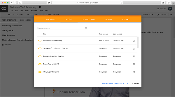
Step 2 − Click on the NEW PYTHON 3 NOTEBOOK link at the bottom of the screen. A new notebook would open up as shown in the screen below.

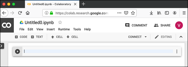
As you might have noticed, the notebook interface is quite similar to the one provided in Jupyter. There is a code window in which you would enter your Python code.

Setting Notebook Name

By default, the notebook uses the naming convention UntitledXX.ipynb. To rename the notebook, click on this name and type in the desired name in the edit box as shown here −

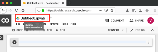
We will call this notebook as MyFirstColabNotebook. So type in this name in the edit box and hit ENTER. The notebook will acquire the name that you have given now.

Entering Code

You will now enter a trivial Python code in the code window and execute it.

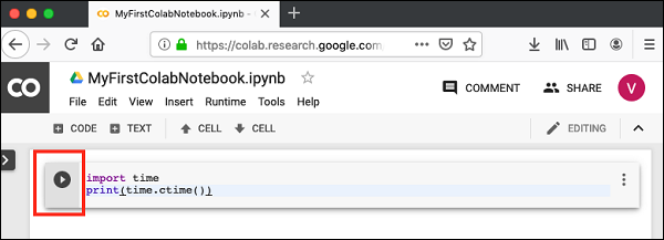
Enter the following two Python statements in the code window −

import time
print(time.ctime())

Executing Code

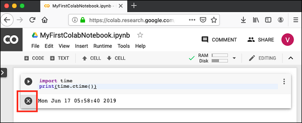
To execute the code, click on the arrow on the left side of the code window.

After a while, you will see the output underneath the code window, as shown here −

Mon Jun 17 05:58:40 2019

You can clear the output anytime by clicking the icon on the left side of the output display.

Adding Code Cells

To add more code to your notebook, select the following menu options −

Insert / Code Cell

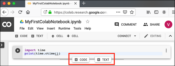
Alternatively, just hover the mouse at the bottom center of the Code cell. When the CODE and TEXT buttons appear, click on the CODE to add a new cell. This is shown in the screenshot below −

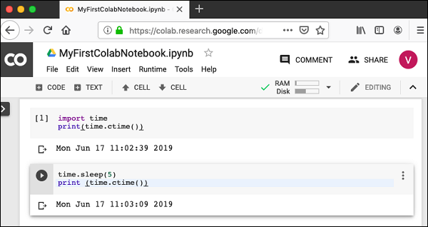
A new code cell will be added underneath the current cell. Add the following two statements in the newly created code window −

time.sleep(5)
print (time.ctime())

Now, if you run this cell, you will see the following output −

Mon Jun 17 04:50:27 2019

Certainly, the time difference between the two time strings is not 5 seconds. This is obvious as you did take some time to insert the new code. Colab allows you to run all code inside your notebook without an interruption.

Run All

To run the entire code in your notebook without an interruption, execute the following menu options −

Runtime / Reset and run all…

It will give you the output as shown below −

Note that the time difference between the two outputs is now exactly 5 seconds.

The above action can also be initiated by executing the following two menu options −

Runtime / Restart runtime…

Runtime / Restart all runtimes…

Followed by

Runtime / Run all

Study the different menu options under the Runtime menu to get yourself acquainted with the various options available to you for executing the notebook.

Changing Cell Order

When your notebook contains a large number of code cells, you may come across situations where you would like to change the order of execution of these cells. You can do so by selecting the cell that you want to move and clicking the UP CELL or DOWN CELL buttons shown in the following screenshot −

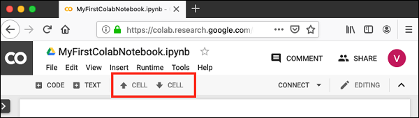
You may click the buttons multiple times to move the cell for more than a single position.

Deleting Cell

During the development of your project, you may have introduced a few now-unwanted cells in your notebook. You can remove such cells from your project easily with a single click. Click on the vertical-dotted icon at the top right corner of your code cell.

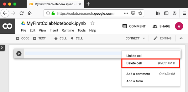
Click on the Delete cell option and the current cell will be deleted.

Now, as you have learned how to run a trivial notebook, let us explore the other capabilities of Colab.

Google Colab - Documenting Your Code

As the code cell supports full Python syntax, you may use Python comments in the code window to describe your code. However, many a time you need more than a simple text based comments to illustrate the ML algorithms. ML heavily uses mathematics and to explain those terms and equations to your readers you need an editor that supports LaTex - a language for mathematical representations. Colab provides Text Cells for this purpose.

A text cell containing few mathematical equations typically used in ML is shown in the screenshot below −

As we move ahead in this chapter, we will see the code for generating the above output.

Text Cells are formatted using markdown - a simple markup language. Let us now see you how to add text cells to your notebook and add to it some text containing mathematical equations.

Markdown Examples

Let us look into few examples of markup language syntax to demonstrate its capabilities.

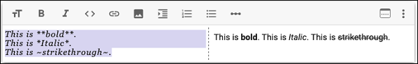
Type in the following text in the Text cell.

This is **bold**.
This is *italic*.
This is ~strikethrough~.

The output of the above commands is rendered on the right hand side of the Cell as shown here.

Mathematical Equations

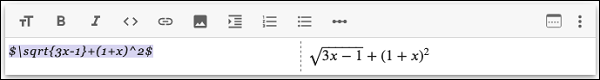
Add a Text Cell to your notebook and enter the following markdown syntax in the text window −

$\sqrt{3x-1}+(1+x)^2$

You will see the immediate rendering of the markdown code in the right hand side panel of the text cell. This is shown in the screenshot below −

Hit Enter and the markdown code disappears from the text cell and only the rendered output is shown.

Let us try another more complicated equation as shown here −

$e^x = \sum_{i = 0}^\infty \frac{1}{i!}x^i$

The rendered output is shown here for your quick reference.

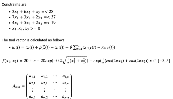
Code for Sample Equations

Here is the code for the sample equations shown in an earlier screenshot −

Constraints are
   - $3x_1 + 6x_2 + x_3 =< 28$
   - $7x_1 + 3x_2 + 2x_3 =< 37$
   - $4x_1 + 5x_2 + 2x_3 =< 19$
   - $x_1,x_2,x_3 >=0 $

The trial vector is calculated as follows:
- $u_i(t) = x_i(t) + \beta(\hat{x}(t) − x_i(t)) + \beta \sum_{k = 1}^{n_v}(x_{i1,k}(t) − x_{i2,k}(t))$
$f(x_1, x_2) = 20 + e - 20exp(-0.2 \sqrt {\frac {1}{n} (x_1^2 + x_2^2)}) - exp (\frac {1}{n}(cos(2\pi x_1) + cos(2\pi x_2))$

$x ∈ [-5, 5]$
>$A_{m,n} =
   \begin{pmatrix}
   a_{1,1} > a_{1,2} > \cdots > a_{1,n} \\
   a_{2,1} > a_{2,2} > \cdots > a_{2,n} \\
   \vdots > \vdots > \ddots > \vdots \\
   a_{m,1} > a_{m,2} > \cdots > a_{m,n}
   \end{pmatrix}$

Describing full markup syntax is beyond the scope of this tutorial. In the next chapter, we will see how to save your work.

Google Colab - Saving Your Work

Colab allows you to save your work to Google Drive or even directly to your GitHub repository.

Saving to Google Drive

Colab allows you to save your work to your Google Drive. To save your notebook, select the following menu options −

File / Save a copy in Drive…

You will see the following screen −

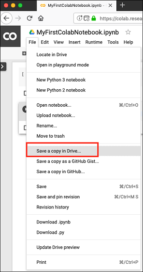
The action will create a copy of your notebook and save it to your drive. Later on you may rename the copy to your choice of name.

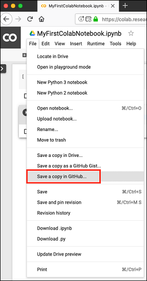
Saving to GitHub

You may also save your work to your GitHub repository by selecting the following menu options −

File / Save a copy in GitHub...

The menu selection is shown in the following screenshot for your quick reference −

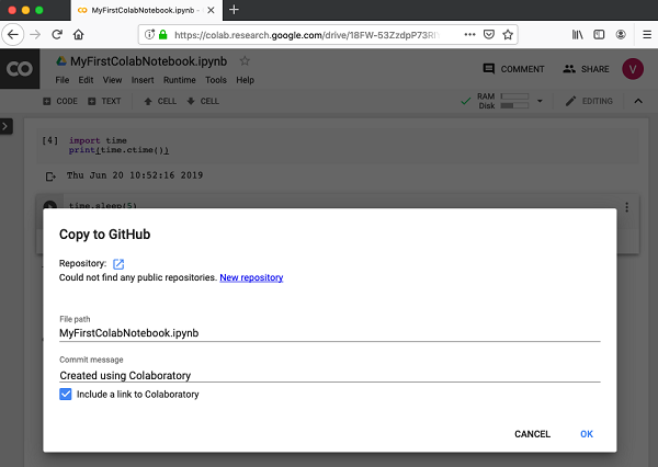
You will have to wait until you see the login screen to GitHub.

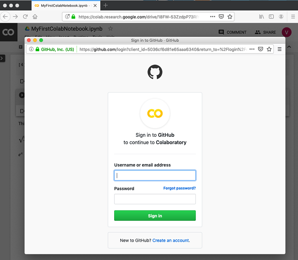
Now, enter your credentials. If you do not have a repository, create a new one and save your project as shown in the screenshot below −

In the next chapter, we will learn how to share your work with others.

Google Colab - Sharing Notebook

To share the notebook that you have created with other co-developers, you may share the copy that you have made in your Google Drive.

To publish the notebook to general audience, you may share it from your GitHub repository.

There is one more way to share your work and that is by clicking on the SHARE link at the top right hand corner of your Colab notebook. This will open the share box as shown here −

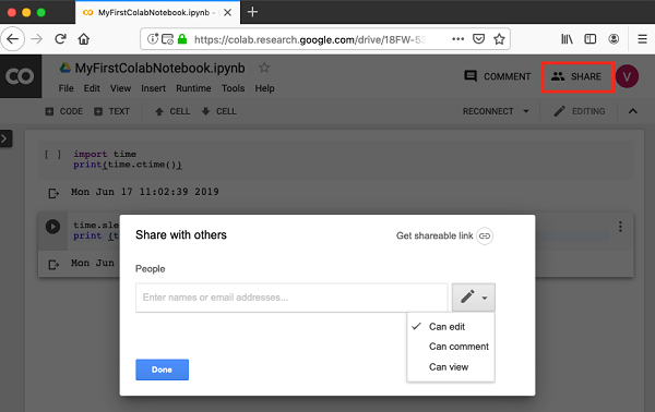
You may enter the email IDs of people with whom you would like to share the current document. You can set the kind of access by selecting from the three options shown in the above screen.

Click on the Get shareable link option to get the URL of your notebook. You will find options for whom to share as follows −

Specified group of people
Colleagues in your organization
Anyone with the link
All public on the web

Now. you know how to create/execute/save/share a notebook. In the Code cell, we used Python so far. The code cell can also be used for invoking system commands. This is explained next.

Google Colab - Invoking System Commands

Jupyter includes shortcuts for many common system operations. Colab Code cell supports this feature.

Simple Commands

Enter the following code in the Code cell that uses the system command echo.

message = 'A Great Tutorial on Colab by Tutorialspoint!'
greeting = !echo -e '$message\n$message'
greeting

Now, if you run the cell, you will see the following output −

['A Great Tutorial on Colab by Tutorialspoint!', 'A Great Tutorial on Colab by Tutorialspoint!']

Getting Remote Data

Let us look into another example that loads the dataset from a remote server. Type in the following command in your Code cell −

!wget http://mlr.cs.umass.edu/ml/machine-learning-databases/adult/adult.data -P "/content/drive/My Drive/app"

If you run the code, you would see the following output −

--2019-06-20 10:09:53-- http://mlr.cs.umass.edu/ml/machine-learning-databases/adult/adult.data
Resolving mlr.cs.umass.edu (mlr.cs.umass.edu)... 128.119.246.96
Connecting to mlr.cs.umass.edu (mlr.cs.umass.edu)|128.119.246.96|:80... connected. 
HTTP request sent, awaiting response... 200 OK 
Length: 3974305 (3.8M) [text/plain] 
Saving to: ‘/content/drive/My Drive/app/adult.data.1’

adult.data.1 100%[===================>] 3.79M 1.74MB/s in 2.2s

2019-06-20 10:09:56 (1.74 MB/s) - ‘/content/drive/My Drive/app/adult.data.1’ saved [3974305/3974305]

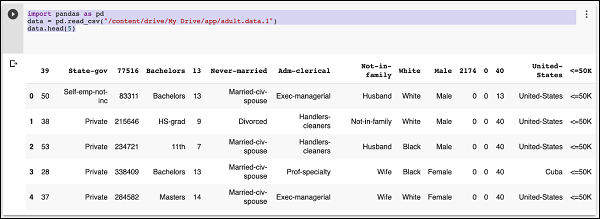
As the message says, the adult.data.1 file is now added to your drive. You can verify this by examining the folder contents of your drive. Alternatively, type in the following code in a new Code cell −

import pandas as pd
data = pd.read_csv("/content/drive/My Drive/app/adult.data.1")
data.head(5)

Run the code now and you will see the following output −

Likewise, most of the system commands can be invoked in your code cell by prepending the command with an Exclamation Mark (!). Let us look into another example before giving out the complete list of commands that you can invoke.

Cloning Git Repository

You can clone the entire GitHub repository into Colab using the gitcommand. For example, to clone the keras tutorial, type the following command in the Code cell −

!git clone https://github.com/wxs/keras-mnist-tutorial.git

After a successful run of the command, you would see the following output −

Cloning into 'keras-mnist-tutorial'...
remote: Enumerating objects: 26, done.
remote: Total 26 (delta 0), reused 0 (delta 0), pack-reused 26
Unpacking objects: 100% (26/26), done.

Once the repo is cloned, locate a Jupyter project (e.g. MINST in keras.ipyab) in it, right-click on the file name and select Open With / Colaboratory menu option to open the project in Colab.

System Aliases

To get a list of shortcuts for common operations, execute the following command −

!ls /bin

You will see the list in the output window as shown below −

bash*             journalctl*       sync*
bunzip2*          kill*             systemctl*
bzcat*            kmod*             systemd@
bzcmp@            less*             systemd-ask-password*
bzdiff*           lessecho*         systemd-escape*
bzegrep@          lessfile@         systemd-hwdb*
bzexe*            lesskey*          systemd-inhibit*
bzfgrep@          lesspipe*         systemd-machine-id-setup*
bzgrep*           ln*               systemd-notify*
bzip2*            login*            systemd-sysusers*
bzip2recover*     loginctl*         systemd-tmpfiles*
bzless@           ls*               systemd-tty-ask-password-agent*
bzmore*           lsblk*            tar*
cat*              lsmod@            tempfile*
chgrp*            mkdir*            touch*
chmod*            mknod*            true*
chown*            mktemp*           udevadm*
cp*               more*             ulockmgr_server*
dash*             mount*            umount*
date*             mountpoint*       uname*
dd*               mv*               uncompress*
df*               networkctl*       vdir*
dir*              nisdomainname@    wdctl*
dmesg*            pidof@            which*
dnsdomainname@    ps*               ypdomainname@
domainname@       pwd*              zcat*
echo*             rbash@            zcmp*
egrep*            readlink*         zdiff*
false*            rm*               zegrep*
fgrep*            rmdir*            zfgrep*
findmnt*          run-parts*        zforce*
fusermount*       sed*              zgrep*
grep*             sh@               zless*
gunzip*           sh.distrib@       zmore*
gzexe*            sleep*            znew*
gzip*             stty*
hostname*         su*

Execute any of these commands as we have done for echo and wget. In the next chapter, we shall see how to execute your previously created Python code.

Google Colab - Executing External Python Files

Suppose, you already have some Python code developed that is stored in your Google Drive. Now, you will like to load this code in Colab for further modifications. In this chapter, we will see how to load and run the code stored in your Google Drive.

Mounting Drive

Tools / Command palette

You will see the list of commands as shown in this screenshot −

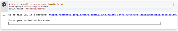
Type a few letters like “m” in the search box to locate the mount command. Select Mount Drive command from the list. The following code would be inserted in your Code cell.

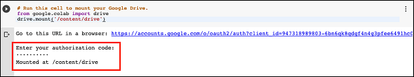
# Run this cell to mount your Google Drive.
from google.colab import drive
drive.mount('/content/drive')

If you run this code, you will be asked to enter the authentication code. The corresponding screen looks as shown below −

Open the above URL in your browser. You will be asked to login to your Google account. Now, you will see the following screen −

If you grant the permissions, you will receive your code as follows −

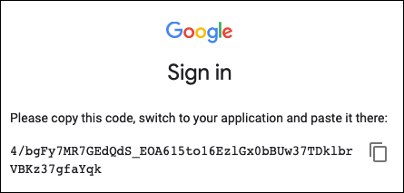
Cut-n-paste this code in the Code cell and hit ENTER. After a while, the drive will be mounted as seen in the screenshot below −

Now, you are ready to use the contents of your drive in Colab.

Listing Drive Contents

You can list the contents of the drive using the ls command as follows −

!ls "/content/drive/My Drive/Colab Notebooks"

This command will list the contents of your Colab Notebooks folder. The sample output of my drive contents are shown here −

Greeting.ipynb hello.py LogisticRegressionCensusData.ipynb LogisticRegressionDigitalOcean.ipynb MyFirstColabNotebook.ipynb SamplePlot.ipynb

Running Python Code

Now, let us say that you want to run a Python file called hello.py stored in your Google Drive. Type the following command in the Code cell −

!python3 "/content/drive/My Drive/Colab Notebooks/hello.py"

The contents of hello.py are given here for your reference −

print("Welcome to TutorialsPoint!")

You will now see the following output −

Welcome to TutorialsPoint!

Besides the text output, Colab also supports the graphical outputs. We will see this in the next chapter.

Google Colab - Graphical Outputs

Colab also supports rich outputs such as charts. Type in the following code in the Code cell.

import numpy as np
from matplotlib import pyplot as plt

y = np.random.randn(100)
x = [x for x in range(len(y))]

plt.plot(x, y, '-')
plt.fill_between(x, y, 200, where = (y > 195), facecolor='g', alpha=0.6)

plt.title("Sample Plot")
plt.show()

Now, if you run the code, you will see the following output −

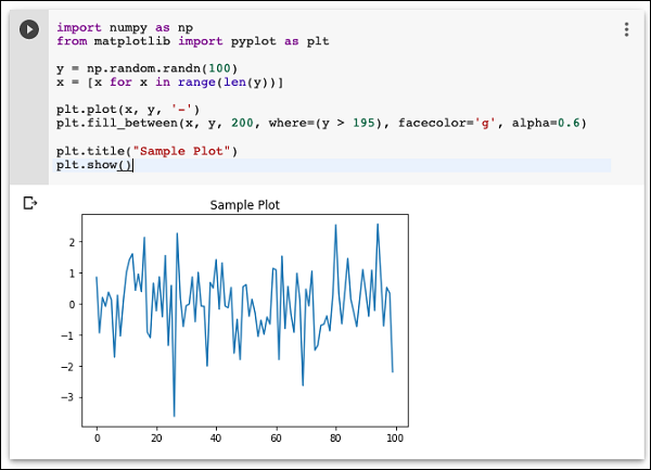
Note that the graphical output is shown in the output section of the Code cell. Likewise, you will be able to create and display several types of charts throughout your program code.

Now, as you have got familiar with the basics of Colab, let us move on to the features in Colab that makes your Python code development easier.

Google Colab - Code Editing Help

The present day developers rely heavily on context-sensitive help to the language and library syntaxes. That is why the IDEs are widely used. The Colab notebook editor provides this facility.

In this chapter, let us see how to ask for context-sensitive help while writing Python code in Colab. Follow the steps that have been given wherever needed.

Function List

Step 1 − Open a new notebook and type in the following code in the Code cell −

import torch

Step 2 − Run the code by clicking on the Run icon in the left panel of the Code cell. Add another Code cell and type in the following code −

Tensor = torch.

At this point, suppose you have forgotten what are the various functions available in torch module. You can ask for the context-sensitive help on function names by hitting the TAB key. Note the presence of the DOT after the torch keyword. Without this DOT, you will not see the context help. Your screen would look like as shown in the screenshot here −

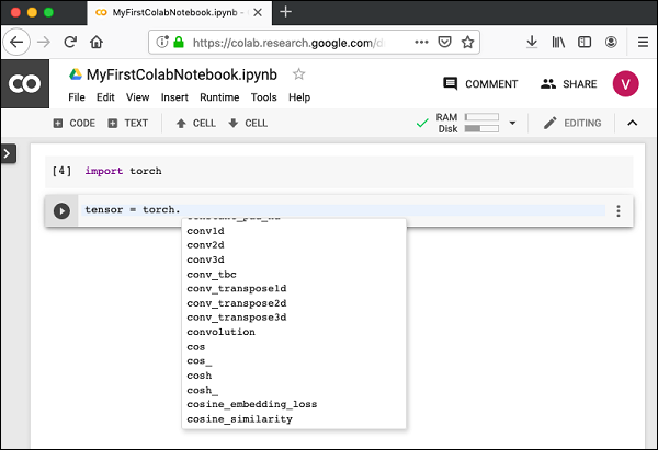
Now, select the desired function from the list and proceed with your coding.

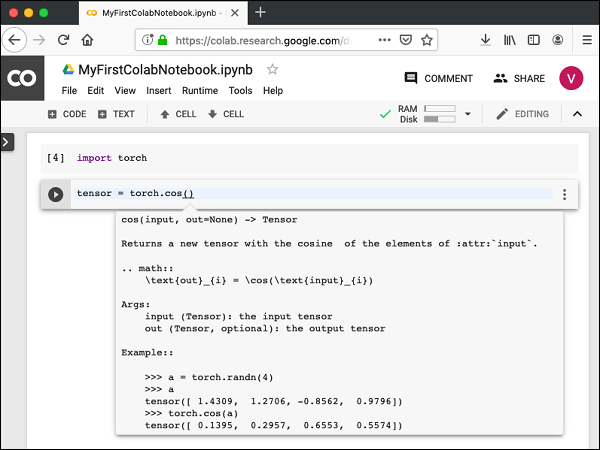
Function Documentation

Colab gives you the documentation on any function or class as a context-sensitive help.

Type the following code in your code window −

Tensor = torch.cos(

Now, hit TAB and you will see the documentation on cos in the popup window as shown in the screenshot here. Note that you need to type in open parenthesis before hitting TAB.

In the next chapter, we will see Magics in Colab that lets us to do more powerful things than what we did with system aliases.

Google Colab - Magics

Magics is a set of system commands that provide a mini extensive command language.

Magics are of two types −

Line magics
Cell magics

The line magics as the name indicates that it consists of a single line of command, while the cell magic covers the entire body of the code cell.

In case of line magics, the command is prepended with a single % character and in the case of cell magics, it is prepended with two % characters (%%).

Let us look into some examples of both to illustrate these.

Line Magics

Type the following code in your code cell −

%ldir

You will see the contents of your local directory, something like this -

drwxr-xr-x 3 root 4096 Jun 20 10:05 drive/
drwxr-xr-x 1 root 4096 May 31 16:17 sample_data/

Try the following command −

%history

This presents the complete history of commands that you have previously executed.

Cell Magics

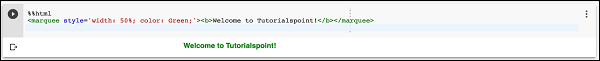
Type in the following code in your code cell −

%%html
<marquee style='width: 50%; color: Green;'>Welcome to Tutorialspoint!</marquee>

Now, if you run the code and you will see the scrolling welcome message on the screen as shown here −

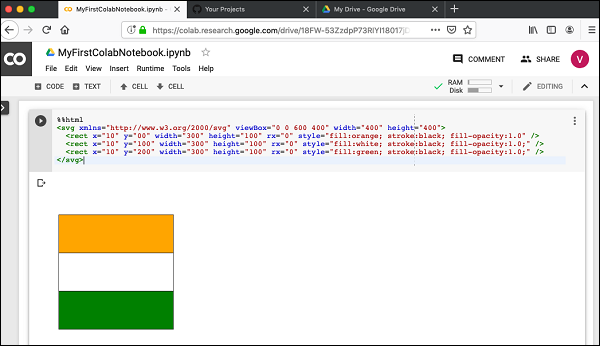
The following code will add SVG to your document.

%%html
<svg xmlns="https://www.w3.org/2000/svg" viewBox="0 0 600 400" width="400" height="400">
   <rect x="10" y="00" width="300" height="100" rx="0" style="fill:orange; stroke:black; fill-opacity:1.0" />
   <rect x="10" y="100" width="300" height="100" rx="0" style="fill:white; stroke:black; fill-opacity:1.0;" />
   <rect x="10" y="200" width="300" height="100" rx="0" style="fill:green; stroke:black; fill-opacity:1.0;" />
</svg>

If you run the code, you would see the following output −

Magics List

To get a complete list of supported magics, execute the following command −

%lsmagic

You will see the following output −

Available line magics:
%alias %alias_magic %autocall %automagic %autosave %bookmark %cat %cd %clear
%colors %config %connect_info %cp %debug %dhist %dirs %doctest_mode %ed %edit
%env %gui %hist %history %killbgscripts %ldir %less %lf %lk %ll %load %load_ext
%loadpy %logoff %logon %logstart %logstate %logstop %ls %lsmagic %lx %macro
%magic %man %matplotlib %mkdir %more %mv %notebook %page %pastebin %pdb %pdef
%pdoc %pfile %pinfo %pinfo2 %pip %popd %pprint %precision %profile %prun
%psearch %psource %pushd %pwd %pycat %pylab %qtconsole %quickref %recall
%rehashx %reload_ext %rep %rerun %reset %reset_selective %rm %rmdir %run %save
%sc %set_env %shell %store %sx %system %tb %tensorflow_version %time %timeit
%unalias %unload_ext %who %who_ls %whos %xdel %xmode

Available cell magics:
%%! %%HTML %%SVG %%bash %%bigquery %%capture %%debug %%file %%html %%javascript
%%js %%latex %%perl %%prun %%pypy %%python %%python2 %%python3 %%ruby %%script
%%sh %%shell %%svg %%sx %%system %%time %%timeit %%writefile

Automagic is ON, % prefix IS NOT needed for line magics.

Next, you will learn another powerful feature in Colab to set the program variables at runtime.

Google Colab - Adding Forms

Colab provides a very useful utility called Forms that allows you to accept inputs from the user at runtime. Let us now move on to see how to add forms to your notebook.

Adding Form

In an earlier lesson, you used the following code to create a time delay −

import time
print(time.ctime())
time.sleep(5)
print (time.ctime())

Suppose, you want a user set time delay instead of a fixed delay of 5 seconds. For this, you can add a Form to the Code cell to accept the sleep time.

Open a new notebook. Click on the Options (vertically-dotted) menu. A popup menu shows up as seen in the screenshot below −

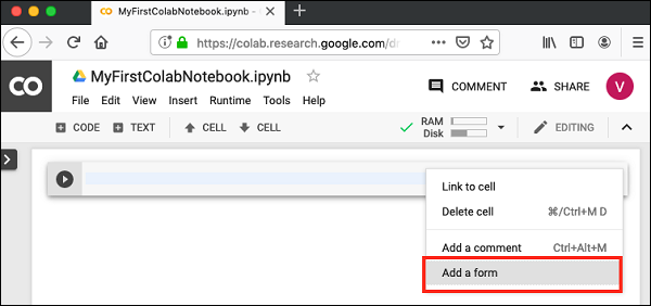
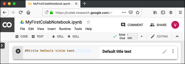
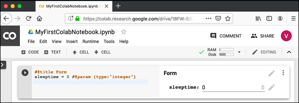
Now, select Add a form option. It will add the form to your Code cell with a Default title as seen in the screenshot here −

To change the title of the form, click on the Settings button (pencil icon on the right). It will pop up a settings screen as shown here:

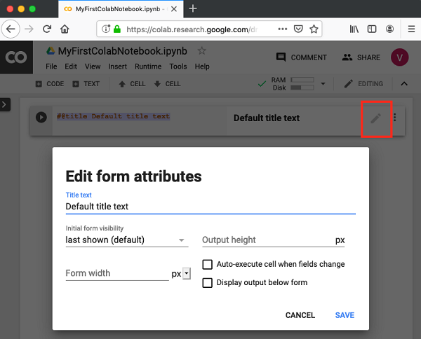
Change the form title to “Form” and save the form. You may use some other name of your choice. Notice that it adds the @title to your code cell.

You may explore other options on the above screen at a later time. In the next section, we will learn how add input fields to the form.

Adding Form Fields

To add a form field, click the Options menu in the Code cell, click on the Form to reveal the submenus. The screen will look as shown below −

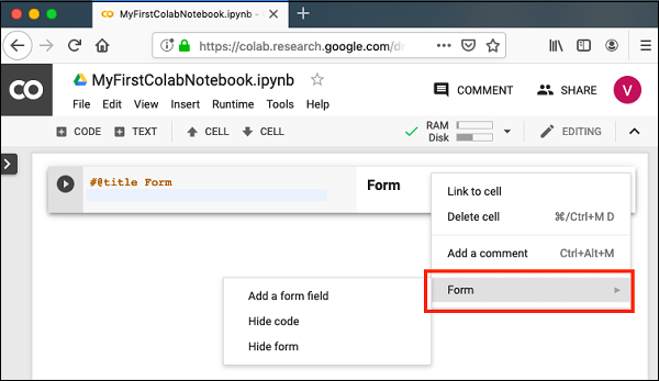
Select Add a form field menu option. A dialog pops up as seen here −

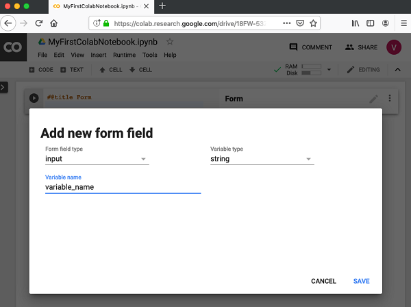
Leave the Form field type to input. Change the Variable name to sleeptime and set the Variable type to integer. Save the changes by clicking the Save button.

Your screen will now look like the following with the sleeptime variable added into the code.

Next, let us see how to test the form by adding some code that uses the sleeptime variable.

Testing Form

Add a new Code cell underneath the form cell. Use the code given below −

import time
print(time.ctime())
time.sleep(sleeptime)
print (time.ctime())

You have used this code in the earlier lesson. It prints the current time, waits for a certain amount of time and prints a new timestamp. The amount of time that the program waits is set in the variable called sleeptime.

Now, go back to the Form Cell and type in a value of 2 for the sleeptime. Select the following menu −

Runtime / Run all

This runs the entire notebook. You can see an output screen as shown below.

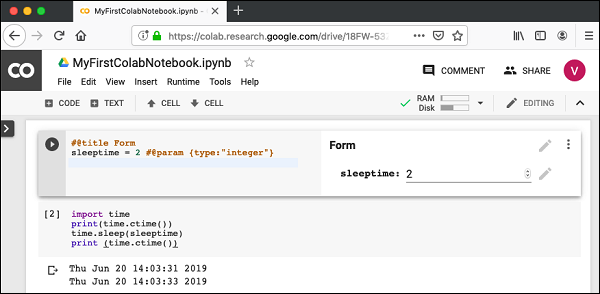
Notice that it has taken your input value of 2 for the

sleeptime

. Try changing this to a different value and Run all to see its effect.

Inputting Text

To accept a text input in your form, enter the following code in a new code cell.

name = 'Tutorialspoint' #@param {type:"string"}
print(name)

Now, if you run the Code cell, whatever the name you set in the form would be printed on the screen. By default, the following output would appear on the screen.

Tutorialspoint

Note that you may use the menu options as shown for the integer input to create a Text input field.

Dropdown List

To add a dropdown list to your form, use the following code −

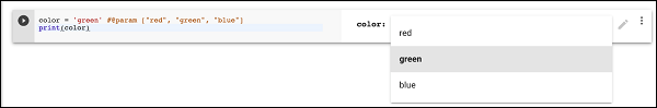
color = 'green' #@param ["red", "green", "blue"]
print(color)

This creates a dropdown list with three values - red, green and blue. The default selection is green.

The dropdown list is shown in the screenshot below −

Date Input

Colab Form allows you to accept dates in your code with validations. Use the following code to input date in your code.

#@title Date fields
date_input = '2019-06-03' #@param {type:"date"}
print(date_input)

The Form screen looks like the following.

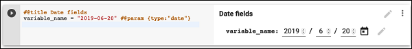
Try inputting a wrong date value and observe the validations.

So far you have learned how to use Colab for creating and executing Jupyter notebooks with your Python code. In the next chapter, we will see how to install popular ML libraries in your notebook so that you can use those in your Python code.

Google Colab - Installing ML Libraries

Colab supports most of machine learning libraries available in the market. In this chapter, let us take a quick overview of how to install these libraries in your Colab notebook.

To install a library, you can use either of these options −

!pip install

!apt-get install

Keras

Keras, written in Python, runs on top of TensorFlow, CNTK, or Theano. It enables easy and fast prototyping of neural network applications. It supports both convolutional networks (CNN) and recurrent networks, and also their combinations. It seamlessly supports GPU.

To install Keras, use the following command −

!pip install -q keras

PyTorch

PyTorch is ideal for developing deep learning applications. It is an optimized tensor library and is GPU enabled. To install PyTorch, use the following command −

!pip3 install torch torchvision

MxNet

Apache MxNet is another flexible and efficient library for deep learning. To install MxNet execute the following commands −

!apt install libnvrtc8.0
!pip install mxnet-cu80

OpenCV

OpenCV is an open source computer vision library for developing machine learning applications. It has more than 2500 optimized algorithms which support several applications such as recognizing faces, identifying objects, tracking moving objects, stitching images, and so on. Giants like Google, Yahoo, Microsoft, Intel, IBM, Sony, Honda, Toyota use this library. This is highly suited for developing real-time vision applications.

To install OpenCV use the following command −

!apt-get -qq install -y libsm6 libxext6 && pip install -q -U opencv-python

XGBoost

XGBoost is a distributed gradient boosting library that runs on major distributed environments such as Hadoop. It is highly efficient, flexible and portable. It implements ML algorithms under the Gradient Boosting framework.

To install XGBoost, use the following command −

!pip install -q xgboost==0.4a30

GraphViz

Graphviz is an open source software for graph visualizations. It is used for visualization in networking, bioinformatics, database design, and for that matter in many domains where a visual interface of the data is desired.

To install GraphViz, use the following command −

!apt-get -qq install -y graphviz && pip install -q pydot

By this time, you have learned to create Jupyter notebooks containing popular machine learning libraries. You are now ready to develop your machine learning models. This requires high processing power. Colab provides free GPU for your notebooks.

In the next chapter, we will learn how to enable GPU for your notebook.

Google Colab - Using Free GPU

Google provides the use of free GPU for your Colab notebooks.

Enabling GPU

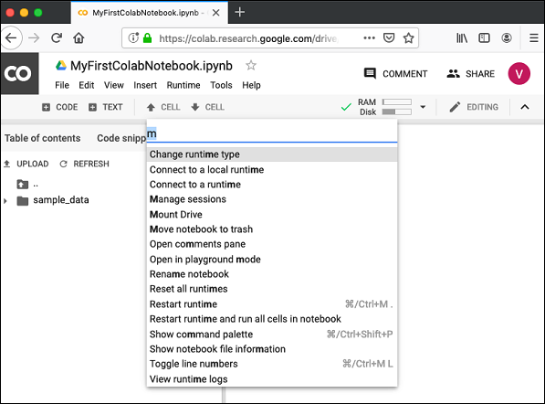
To enable GPU in your notebook, select the following menu options −

Runtime / Change runtime type

You will see the following screen as the output −

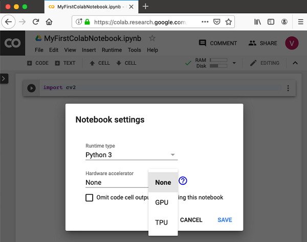
Select GPU and your notebook would use the free GPU provided in the cloud during processing. To get the feel of GPU processing, try running the sample application from MNIST tutorial that you cloned earlier.

!python3 "/content/drive/My Drive/app/mnist_cnn.py"

Try running the same Python file without the GPU enabled. Did you notice the difference in speed of execution?

Testing for GPU

You can easily check if the GPU is enabled by executing the following code −

import tensorflow as tf
tf.test.gpu_device_name()

If the GPU is enabled, it will give the following output −

'/device:GPU:0'

Listing Devices

If you are curious to know the devices used during the execution of your notebook in the cloud, try the following code −

from tensorflow.python.client import device_lib
device_lib.list_local_devices()

You will see the output as follows −

[name: "/device:CPU:0"
   device_type: "CPU"
   memory_limit: 268435456
   locality { }
   incarnation: 1734904979049303143, name: "/device:XLA_CPU:0"
   device_type: "XLA_CPU" memory_limit: 17179869184
   locality { } 
   incarnation: 16069148927281628039
   physical_device_desc: "device: XLA_CPU device", name: "/device:XLA_GPU:0"
   device_type: "XLA_GPU"
   memory_limit: 17179869184
   locality { }
   incarnation: 16623465188569787091
   physical_device_desc: "device: XLA_GPU device", name: "/device:GPU:0"
   device_type: "GPU"
   memory_limit: 14062547764
   locality {
      bus_id: 1
      links { } 
   }
   incarnation: 6674128802944374158
physical_device_desc: "device: 0, name: Tesla T4, pci bus id: 0000:00:04.0, compute capability: 7.5"]

Checking RAM

To see the memory resources available for your process, type the following command −

!cat /proc/meminfo

You will see the following output −

MemTotal: 13335276 kB
MemFree: 7322964 kB
MemAvailable: 10519168 kB
Buffers: 95732 kB
Cached: 2787632 kB
SwapCached: 0 kB
Active: 2433984 kB
Inactive: 3060124 kB
Active(anon): 2101704 kB
Inactive(anon): 22880 kB
Active(file): 332280 kB
Inactive(file): 3037244 kB
Unevictable: 0 kB
Mlocked: 0 kB
SwapTotal: 0 kB
SwapFree: 0 kB
Dirty: 412 kB
Writeback: 0 kB
AnonPages: 2610780 kB
Mapped: 838200 kB
Shmem: 23436 kB
Slab: 183240 kB
SReclaimable: 135324 kB
SUnreclaim: 47916
kBKernelStack: 4992 kB
PageTables: 13600 kB
NFS_Unstable: 0 kB
Bounce: 0 kB
WritebackTmp: 0 kB
CommitLimit: 6667636 kB
Committed_AS: 4801380 kB
VmallocTotal: 34359738367 kB
VmallocUsed: 0 kB
VmallocChunk: 0 kB
AnonHugePages: 0 kB
ShmemHugePages: 0 kB
ShmemPmdMapped: 0 kB
HugePages_Total: 0
HugePages_Free: 0
HugePages_Rsvd: 0
HugePages_Surp: 0
Hugepagesize: 2048 kB
DirectMap4k: 303092 kB
DirectMap2M: 5988352 kB
DirectMap1G: 9437184 kB

You are now all set for the development of machine learning models in Python using Google Colab.

Google Colab - Conclusion

Google Colab is a powerful platform for learning and quickly developing machine learning models in Python. It is based on Jupyter notebook and supports collaborative development. The team members can share and concurrently edit the notebooks, even remotely. The notebooks can also be published on GitHub and shared with the general public. Colab supports many popular ML libraries such as PyTorch, TensorFlow, Keras and OpenCV. The restriction as of today is that it does not support R or Scala yet. There is also a limitation to sessions and size. Considering the benefits, these are small sacrifices one needs to make.