- Excel Charts - Home
- Excel Charts - Introduction
- Excel Charts - Creating Charts
- Excel Charts - Types
- Excel Charts - Column Chart
- Excel Charts - Line Chart
- Excel Charts - Pie Chart
- Excel Charts - Doughnut Chart
- Excel Charts - Bar Chart
- Excel Charts - Area Chart
- Excel Charts - Scatter (X Y) Chart
- Excel Charts - Bubble Chart
- Excel Charts - Stock Chart
- Excel Charts - Surface Chart
- Excel Charts - Radar Chart
- Excel Charts - Combo Chart
- Excel Charts - Chart Elements
- Excel Charts - Chart Styles
- Excel Charts - Chart Filters
- Excel Charts - Fine Tuning
- Excel Charts - Design Tools
- Excel Charts - Quick Formatting
- Excel Charts - Aesthetic Data Labels
- Excel Charts - Format Tools
- Excel Charts - Sparklines
- Excel Charts - PivotCharts
Excel Charts - Quick Formatting
You can format charts quickly using the Format pane. It is quite handy and provides advanced formatting options.
To Format any chart element,
Step 1 − Click on the chart.
Step 2 − Right-click chart element.
Step 3 − Click Format <Chart Element> from the drop-down list.
The Format pane appears with options that are tailored for the selected chart element.
Format Pane
The Format pane by default appears on the right-side of the chart.
Step 1 − Click on the chart.
Step 2 − Right-click the horizontal axis. A drop-down list appears.
Step 3 − Click Format Axis. The Format pane for formatting axis appears. The format pane contains the task pane options.
Step 4 − Click the ![]() Task Pane Options icon.
Task Pane Options icon.
The task pane options Move, Size or Close appear in the drop-down. You can move, resize or close the format pane using these options.
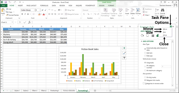
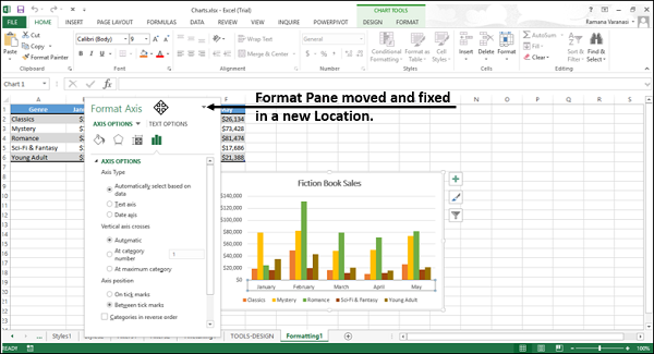
Step 5 − Click Move. The mouse pointer changes to  holding which you can move the Format Pane. Drag the format pane to the location you want.
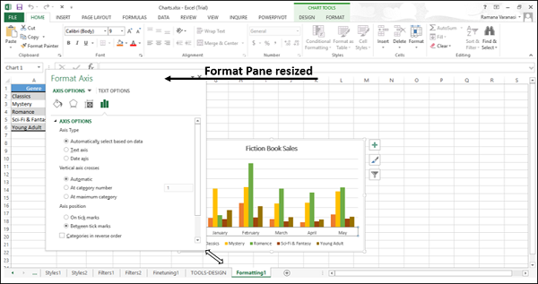
Step 6 − Click the Size option from the task pane options to resize the format window. The pointer changes to an arrow, which appears at the right-bottom corner of the format pane.
Step 7 − Click Close from the task pane options.
The Format Pane closes.
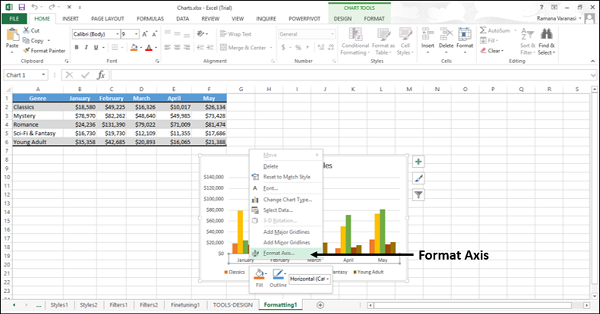
Format Axis
To format axis quickly follow the steps given below.
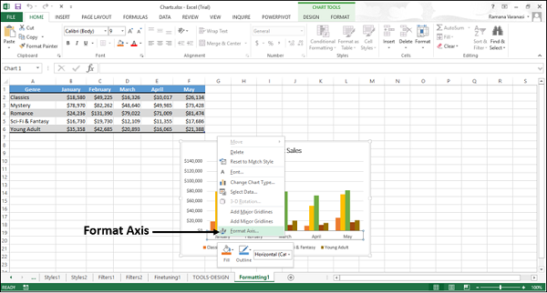
Step 1 − Right-click the chart axis and then click Format Axis.
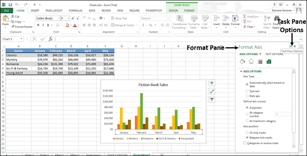
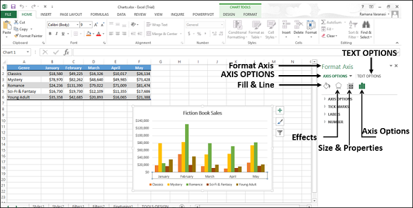
The Format Axis pane appears.
In the Format Axis pane, you will see two tabs −
- AXIS OPTIONS
- TEXT OPTIONS
By default, Axis Options are highlighted. The icons below these options on the pane are to format the appearance of the axes.
Step 2 − Click Axis Options. The various available options for formatting axis will appear.
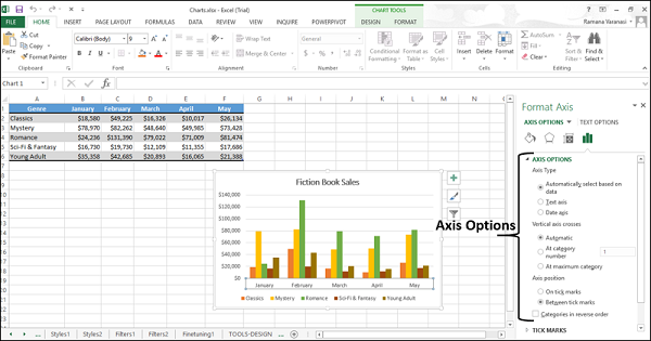
Step 3 − Select the required Axis Options. You can edit the display of the axes through these options.
Format Chart Title
To format the chart title, follow the steps given below.
Step 1 − Right-click the chart title and then click Format Chart Title.
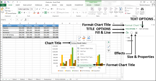
Step 2 − Select the required Title Options.
You can edit the display of the chart title through these options.
Format Chart Area
To format the chart area, follow the steps given below.
Step 1 − Right-click the chart area and then click Format Chart Area.
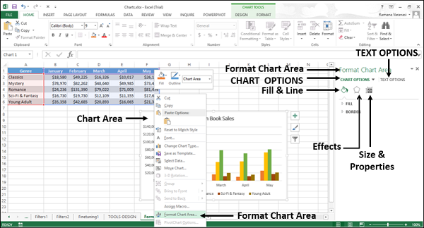
Step 2 − Select the required Chart Options.
You can edit the display of your chart through these options.
Format Plot Area
To format the plot area, follow the steps given below.
Step 1 − Right-click the plot area and then click Format Plot Area.
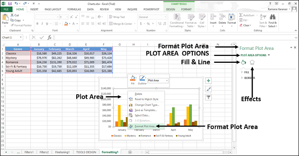
Step 2 − Select the required Plot Area Options.
You can edit the display of the plot area where your chart is plotted through these options.
Format Data Series
To format the data series −
Step 1 − Right-click any of the data series of your chart and then click Format Data Series.
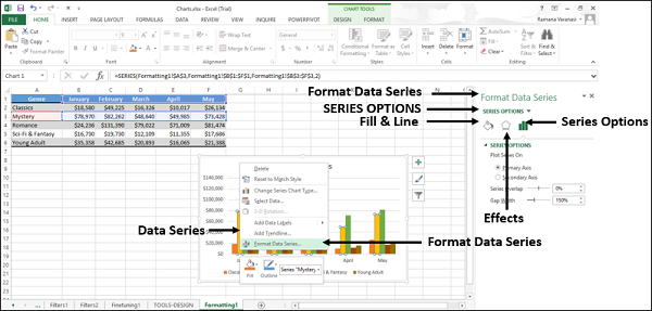
Step 2 − Select the required Series Options.
You can edit the display of the series through these options.
Format Data Labels
To format data labels quickly, follow the steps −
Step 1 − Right-click a data label. The data labels of the entire series are selected. Click Format Data Labels.
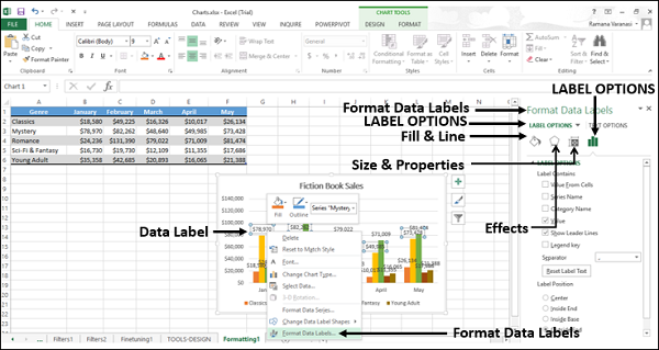
Step 2 − Select the required Label Options.
You can edit the display of the data labels of the selected series through these options.
Format Data Point
To format the data point in your line chart −
Step 1 − Click the data point that you want to format. The data points of the entire series are selected.
Step 2 − Click the data point again. Now, only that particular data point is selected.
Step 3 − Right-click that particular selected data point and then click Format Data Point.
The Format Pane Format Data Point appears.
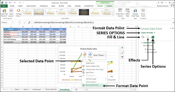
Step 4 − Select the required Series Options. You can edit the display of the data points through these options.
Format Legend
To format Legend −
Step 1 − Right-click legend and then click Format Legend.
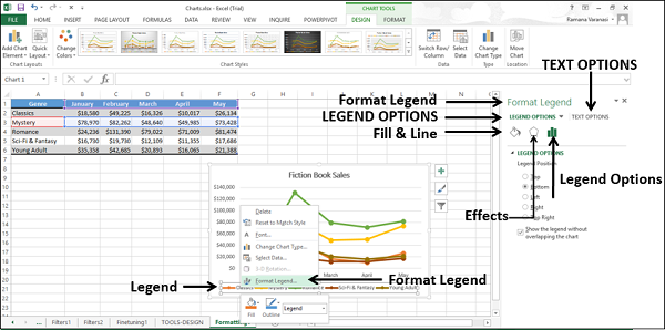
Step 2 − Select the required Legend Options. You can edit the display of the legends through these options.
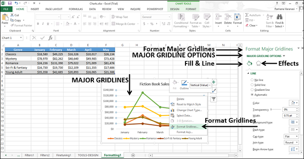
Format Major Gridlines
Format major gridlines of your chart by following the steps given below −
Step 1 − Right-click the major gridlines and then click Format Gridlines.