- Cosmology - Home
- The Expanding Universe
- Cepheid Variables
- Redshift and Recessional Velocity
- Redshift Vs. Kinematic Doppler Shift
- Cosmological Metric & Expansion
- Robertson-Walker Metric
- Hubble Parameter & Scale Factor
- Friedmann Equation & World Models
- Fluid Equation
- Matter Dominated Universe
- Radiation Dominated Universe
- The Dark Energy
- Spiral Galaxy Rotation Curves
- Velocity Dispersion Measurements of Galaxies
- Hubble & Density Parameter
- Age of The Universe
- Angular Diameter Distance
- Luminosity Distance
- Type 1A Supernovae
- Cosmic Microwave Background
- CMB - Temperature at Decoupling
- Anisotropy of CMB Radiation & Cobe
- Modelling the CMB Anisotropies
- Horizon Length at the Surface of Last Scattering
- Extrasolar Planet Detection
- Radial Velocity Method
- Transit Method
- Exoplanet Properties
Cosmology - Transit Method
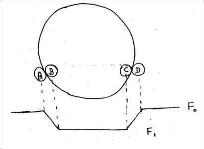
The Transit Method (Kepler Space Telescope) is used to find out the size. The dip in brightness of a star by a planet is usually very less unlike a binary system.
F0 is flux of the star before the planet occults it.
F1 is the flux after the entire planet is in front of star.
The following image will be used for all the calculations.
$$\frac{F_0 - F_1}{F_0} = \frac{\pi r_p^{2}}{\pi R^2_\ast}$$
$$\frac{\Delta F}{F} \cong \frac{r^2_p}{R^2_\ast}$$
$$\left ( \frac{\Delta F}{F} \right )_{earth} \cong 0.001\%$$
$$\left ( \frac{\Delta F}{F} \right )_{jupiter} \cong 1\%$$
This is not easy to achieve by ground based telescope. It is achieved by the Hubble telescope.
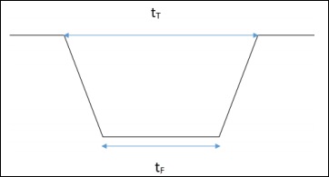
Here, $t_T$ is time between position A and D and $t_F$ is time between position B and C.
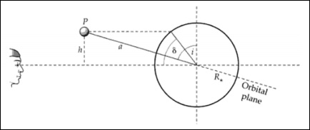
The geometry of a transit related to the inclination i of the system. Transit latitude and inclination are interchangeable.
From the above images, we can write −
$$\frac{h}{a} = cos(i)$$
$$\frac{h}{R_\ast} = sin(\delta)$$
$$cos(i) = \frac{R_\ast sin(\delta)}{a}$$
$$y^2 = (R_\ast + R_p)^2 - h^2$$
$$y = [(R_\ast + R_p)^2 - h^2]^{\frac{1}{2}}$$
$$sin(\theta) = \frac{y}{a}$$
$$\theta = sin^{-1}\left [ \frac{(R_\ast + R_p)^2 - a^2cos^2(i)}{a^2} \right ]^{\frac{1}{2}}$$
$$t_T = \frac{P}{2\pi} \times 2\theta$$
Here, $t_T$ is the fraction of a time-period for which transit happens and (2θ/2π) is fraction of angle for which the transit happens.
$$sin(\frac{t_T\pi}{P}) = \frac{R_\ast}{a}\left [ \left ( 1+ \frac{R_p}{R_\ast}\right )^2 - \left ( \frac{a}{R_\ast}cos(i)\right )^2 \right ]^{\frac{1}{2}}$$
Usually, a >> R∗ >> Rp. So, we can write −
$$sin(\frac{t_T\pi}{P}) = \frac{R_\ast}{a}\left [ 1- \left ( \frac{a}{R_\ast}cos(i) \right )^2\right ]^{\frac{1}{2}}$$
Here, P is the duration between two successive transits. The transit time is very less compared to the orbital time-period. Hence,
$$t_T = \frac{P}{\pi}\left [ \left ( \frac{R_\ast}{a}\right )^2 - cos^2(i)\right ]^{\frac{1}{2}}$$
Here, tT, P, R∗ are the observables, a and i should be found out.
Now,
$$sin(\frac{t_F\pi}{P}) = \frac{R_\ast}{a}\left [\left (1 - \frac{R_p}{R_\ast} \right )^2 - \left ( \frac{a}{R_\ast}cos\:i \right )^2\right ]^{\frac{1}{2}}$$
where, $y^2 = (R_\ast R_p)^2 h^2$.
Let,
$$\frac{\Delta F}{F} = D = \left ( \frac{R_p}{R_\ast} \right )^2$$
Now, we can express,
$$\frac{a}{R_\ast} = \frac{2P}{\pi} D^{\frac{1}{4}}(t^2_T - t^2_F)^{-\frac{1}{2}}$$
For the main sequence stars,
$$R_\ast \propto M^\alpha_\ast$$
$$\frac{R_\ast}{R_0} \propto \left ( \frac{M_\ast}{M_0}\right )^\alpha$$
This gives R∗.
Hence, we get value of a also.
So, we get Rp, ap and even i.
For all this,
$$h \leq R_\ast + R_p$$
$$a\: cos\: i \leq R_\ast + R_p$$
For even ~89 degrees, the transit duration is very small. The planet must be very close to get a sufficient transit time. This gives a tight constraint on i. Once we get i, we can derive mpfrom the radial velocity measurement.
This detection by the transit method is called as chance detection, i.e., probability of observing a transit. Transit probability (probability of observing) calculations are shown below.
The transit probability is related to the solid angle traced out by the two extreme transit configurations, which is −
$$Solid \: angle \:of \:planet \: = 2\pi \left ( \frac{2R_\ast}{a} \right )$$
As well as the total solid angle at a semi-major axis a, or −
$$Solid \:angle \:of \:sphere \: =\: 4\pi$$
The probability is the ratio of these two areas −
$$= \: \frac{area \:of\: sky \: covered \:by\: favourable \: orientation}{area\: of\: sky \:covered\: by\: all\: possible\: orientation\: of\: orbit}$$
$= \frac{4\pi a_pR_\ast}{4\pi a^2_p} = \frac{R_\ast}{a_p}$ $\frac{area\: of\: hollow \: cyclinder}{area\: of\: sphere}$
This probability is independent of the observer.
Points to Remember
- The Transit Method (Kepler Space Telescope) is used to find out the size.
- Detection by Transit Method is a chance detection.
- The planet must be very close to get sufficient transit time.
- Transit probability is related to the solid angle of planet.
- This probability is independent of observer frame of reference.