- Biopython - Home
- Biopython - Introduction
- Biopython - Installation
- Creating Simple Application
- Biopython - Sequence
- Advanced Sequence Operations
- Sequence I/O Operations
- Biopython - Sequence Alignments
- Biopython - Overview of BLAST
- Biopython - Entrez Database
- Biopython - PDB Module
- Biopython - Motif Objects
- Biopython - BioSQL Module
- Biopython - Population Genetics
- Biopython - Genome Analysis
- Biopython - Phenotype Microarray
- Biopython - Plotting
- Biopython - Cluster Analysis
- Biopython - Machine Learning
- Biopython - Testing Techniques
Biopython Resources
Biopython - Quick Guide
Biopython - Introduction
Biopython is the largest and most popular bioinformatics package for Python. It contains a number of different sub-modules for common bioinformatics tasks. It is developed by Chapman and Chang, mainly written in Python. It also contains C code to optimize the complex computation part of the software. It runs on Windows, Linux, Mac OS X, etc.
Basically, Biopython is a collection of python modules that provide functions to deal with DNA, RNA & protein sequence operations such as reverse complementing of a DNA string, finding motifs in protein sequences, etc. It provides lot of parsers to read all major genetic databases like GenBank, SwissPort, FASTA, etc., as well as wrappers/interfaces to run other popular bioinformatics software/tools like NCBI BLASTN, Entrez, etc., inside the python environment. It has sibling projects like BioPerl, BioJava and BioRuby.
Features
Biopython is portable, clear and has easy to learn syntax. Some of the salient features are listed below −
Interpreted, interactive and object oriented.
Supports FASTA, PDB, GenBank, Blast, SCOP, PubMed/Medline, ExPASy-related formats.
Option to deal with sequence formats.
Tools to manage protein structures.
BioSQL − Standard set of SQL tables for storing sequences plus features and annotations.
Access to online services and database, including NCBI services (Blast, Entrez, PubMed) and ExPASY services (SwissProt, Prosite).
Access to local services, including Blast, Clustalw, EMBOSS.
Goals
The goal of Biopython is to provide simple, standard and extensive access to bioinformatics through python language. The specific goals of the Biopython are listed below −
Providing standardized access to bioinformatics resources.
High-quality, reusable modules and scripts.
Fast array manipulation that can be used in Cluster code, PDB, NaiveBayes and Markov Model.
Genomic data analysis.
Advantages
Biopython requires very less code and comes up with the following advantages −
Provides microarray data type used in clustering.
Reads and writes Tree-View type files.
Supports structure data used for PDB parsing, representation and analysis.
Supports journal data used in Medline applications.
Supports BioSQL database, which is widely used standard database amongst all bioinformatics projects.
Supports parser development by providing modules to parse a bioinformatics file into a format specific record object or a generic class of sequence plus features.
Clear documentation based on cookbook-style.
Sample Case Study
Let us check some of the use cases (population genetics, RNA structure, etc.,) and try to understand how Biopython plays an important role in this field −
Population Genetics
Population genetics is the study of genetic variation within a population, and involves the examination and modeling of changes in the frequencies of genes and alleles in populations over space and time.
Biopython provides Bio.PopGen module for population genetics. This module contains all the necessary functions to gather information about classic population genetics.
RNA Structure
Three major biological macromolecules that are essential for our life are DNA, RNA and Protein. Proteins are the workhorses of the cell and play an important role as enzymes. DNA (deoxyribonucleic acid) is considered as the blueprint of the cell. It carries all the genetic information required for the cell to grow, take in nutrients, and propagate. RNA (Ribonucleic acid) acts as DNA photocopy in the cell.
Biopython provides Bio.Sequence objects that represents nucleotides, building blocks of DNA and RNA.
Biopython - Installation
This section explains how to install Biopython on your machine. It is very easy to install and it will not take more than five minutes.
A virtual environment allows us to create an isolated working copy of python for a specific project without affecting the outside setup.
We shall use venv module in Python's standard library to create virtual environment. PIP is included by default in Python version 3.4 or later.
Use the following command to create virtual environment in Windows
D:\biopython>py -m venv myenv
On Ubuntu Linux, update the APT repo and install venv if required before creating virtual environment
mvl@GNVBGL3:~ $ sudo apt update && sudo apt upgrade -y
mvl@GNVBGL3:~ $ sudo apt install python3-venv
Then use the following command to create a virtual environment
mvl@GNVBGL3:~ $ sudo python3 -m venv myenv
You need to activate the virtual environment. On Windows use the command
D:\biopython>cd myenv
D:\biopython\myenv>scripts\activate
(myenv) D:\biopython\myenv>
On Ubuntu Linux, use following command to activate the virtual environment
mvl@GNVBGL3:~$ cd myenv
mvl@GNVBGL3:~/myenv$ source bin/activate
(myenv) mvl@GNVBGL3:~/myenv$
Name of the virtual environment appears in the parenthesis. Now that it is activated, we can now install BioPython in it.
D:\biopython\myenv> pip3 install biopython

(myenv) D:\biopython\myenv>pip3 install biopython
Collecting biopython
  Obtaining dependency information for biopython from https://files.pythonhosted.org/packages/a9/13/00db03b01e54070d5b0ec9c71eef86e61afa733d9af76e5b9b09f5dc9165/biopython-1.86-cp312-cp312-win_amd64.whl.metadata
  Downloading biopython-1.86-cp312-cp312-win_amd64.whl.metadata (13 kB)
Collecting numpy (from biopython)
  Obtaining dependency information for numpy from https://files.pythonhosted.org/packages/2d/57/8aeaf160312f7f489dea47ab61e430b5cb051f59a98ae68b7133ce8fa06a/numpy-2.3.5-cp312-cp312-win_amd64.whl.metadata
  Downloading numpy-2.3.5-cp312-cp312-win_amd64.whl.metadata (60 kB)
     ━━━━━━━━━━━━━━━━━━━━━━━━━━━━━━━━━━━━━━━━ 60.9/60.9 kB 1.1 MB/s eta 0:00:00
Downloading biopython-1.86-cp312-cp312-win_amd64.whl (2.7 MB)
   ━━━━━━━━━━━━━━━━━━━━━━━━━━━━━━━━━━━━━━━━ 2.7/2.7 MB 7.9 MB/s eta 0:00:00
Downloading numpy-2.3.5-cp312-cp312-win_amd64.whl (12.8 MB)
   ━━━━━━━━━━━━━━━━━━━━━━━━━━━━━━━━━━━━━━━━ 12.8/12.8 MB 8.8 MB/s eta 0:00:00
Installing collected packages: numpy, biopython
Successfully installed biopython-1.86 numpy-2.3.5
Verify Biopython Installation
Now, you have successfully installed Biopython on your machine. To verify that Biopython is installed properly, type the below command on your python console −
(myenv) D:\biopython\myenv>py
Python 3.12.1 (tags/v3.12.1:2305ca5, Dec  7 2023, 22:03:25) [MSC v.1937 64 bit (AMD64)] on win32
Type "help", "copyright", "credits" or "license" for more information.
>>> import Bio
>>> print(Bio.__version__)
1.86
>>>
It shows the version of Biopython.
As of now, the latest version is biopython-1.86.
Biopython - Creating Simple Application
Let us create a simple Biopython application to parse a bioinformatics file and print the content. This will help us understand the general concept of the Biopython and how it helps in the field of bioinformatics.
example.fasta
Step 1 − First, create a sample sequence file, example.fasta and put the below content into it.
>sp|P25730|FMS1_ECOLI CS1 fimbrial subunit A precursor (CS1 pilin)
MKLKKTIGAMALATLFATMGASAVEKTISVTASVDPTVDLLQSDGSALPNSVALTYSPAV
NNFEAHTINTVVHTNDSDKGVVVKLSADPVLSNVLNPTLQIPVSVNFAGKPLSTTGITID
SNDLNFASSGVNKVSSTQKLSIHADATRVTGGALTAGQYQGLVSIILTKSTTTTTTTKGT

>sp|P15488|FMS3_ECOLI CS3 fimbrial subunit A precursor (CS3 pilin)
MLKIKYLLIGLSLSAMSSYSLAAAGPTLTKELALNVLSPAALDATWAPQDNLTLSNTGVS
NTLVGVLTLSNTSIDTVSIASTNVSDTSKNGTVTFAHETNNSASFATTISTDNANITLDK
NAGNTIVKTTNGSQLPTNLPLKFITTEGNEHLVSGNYRANITITSTIKGGGTKKGTTDKK
The extension, fasta refers to the file format of the sequence file. FASTA originates from the bioinformatics software, FASTA and hence it gets its name. FASTA format has multiple sequence arranged one by one and each sequence will have its own id, name, description and the actual sequence data.
simple_example.py
Step 2 − Create a new python script, *simple_example.py" and enter the below code and save it.
from Bio.SeqIO import parse
from Bio.SeqRecord import SeqRecord
from Bio.Seq import Seq

file = open("example.fasta")

records = parse(file, "fasta")
for record in records:
   print("Id: %s" % record.id)
   print("Name: %s" % record.name)
   print("Description: %s" % record.description)
   print("Annotations: %s" % record.annotations)
   print("Sequence Data: %s" % record.seq)
Let us take a little deeper look into the code −
Line 1 imports the parse class available in the Bio.SeqIO module. Bio.SeqIO module is used to read and write the sequence file in different format and `parse class is used to parse the content of the sequence file.
Line 2 imports the SeqRecord class available in the Bio.SeqRecord module. This module is used to manipulate sequence records and SeqRecord class is used to represent a particular sequence available in the sequence file.
*Line 3" imports Seq class available in the Bio.Seq module. This module is used to manipulate sequence data and Seq class is used to represent the sequence data of a particular sequence record available in the sequence file.
Line 5 opens the example.fasta file using regular python function, open.
Line 7 parse the content of the sequence file and returns the content as the list of SeqRecord object.
Line 9-15 loops over the records using python for loop and prints the attributes of the sequence record (SqlRecord) such as id, name, description, sequence data, etc.
Output
Step 3 − Open a command prompt and go to the folder containing sequence file, example.fasta and run the below command −
> python simple_example.py
Step 4 − Python runs the script and prints all the sequence data available in the sample file, example.fasta. The output will be similar to the following content.
(myenv) D:\biopython\myenv>py simple_example.py
Id: sp|P25730|FMS1_ECOLI
Name: sp|P25730|FMS1_ECOLI
Description: sp|P25730|FMS1_ECOLI CS1 fimbrial subunit A precursor (CS1 pilin)
Annotations: {}
Sequence Data: MKLKKTIGAMALATLFATMGASAVEKTISVTASVDPTVDLLQSDGSALPNSVALTYSPAVNNFEAHTINTVVHTNDSDKGVVVKLSADPVLSNVLNPTLQIPVSVNFAGKPLSTTGITIDSNDLNFASSGVNKVSSTQKLSIHADATRVTGGALTAGQYQGLVSIILTKSTTTTTTTKGT
Id: sp|P15488|FMS3_ECOLI
Name: sp|P15488|FMS3_ECOLI
Description: sp|P15488|FMS3_ECOLI CS3 fimbrial subunit A precursor (CS3 pilin)
Annotations: {}
Sequence Data: MLKIKYLLIGLSLSAMSSYSLAAAGPTLTKELALNVLSPAALDATWAPQDNLTLSNTGVSNTLVGVLTLSNTSIDTVSIASTNVSDTSKNGTVTFAHETNNSASFATTISTDNANITLDKNAGNTIVKTTNGSQLPTNLPLKFITTEGNEHLVSGNYRANITITSTIKGGGTKKGTTDKK
We have seen three classes, parse, SeqRecord and Seq in this example. These three classes provide most of the functionality and we will learn those classes in the coming section.
Biopython - Sequence
A sequence is series of letters used to represent an organisms protein, DNA or RNA. It is represented by Seq class. Seq class is defined in Bio.Seq module.
Lets create a simple sequence in Biopython as shown below −
>>> from Bio.Seq import Seq
>>> seq = Seq("AGCT")
>>> seq
Seq('AGCT')
>>> print(seq)
AGCT
Here, we have created a simple protein sequence AGCT and each letter represents Alanine, Glycine, Cysteine and Threonine.
Each Seq object has one important attribute −
data − the actual sequence string (AGCT)
Also, Biopython exposes all the bioinformatics related configuration data through Bio.Data module. For example, IUPACData.protein_letters has the possible letters of IUPACProtein alphabet.
>>> from Bio.Data import IUPACData
>>> IUPACData.protein_letters
'ACDEFGHIKLMNPQRSTVWY'
Basic Operations
This section briefly explains about all the basic operations available in the Seq class. Sequences are similar to python strings. We can perform python string operations like slicing, counting, concatenation, find, split and strip in sequences.
Use the below codes to get various outputs.
To get the first value in sequence.
>>> seq_string = Seq("AGCTAGCT")
>>> seq_string[0]
'A'
To print the first two values.
>>> seq_string[0:2]
Seq('AG')
To print all the values.
>>> seq_string[ : ]
Seq('AGCTAGCT')
To perform length and count operations.
>>> len(seq_string)
8
>>> seq_string.count('A')
2
To add two sequences.
>>> seq1 = Seq("AGCT")
>>> seq2 = Seq("TCGA")
>>> seq1+seq2
Seq('AGCTTCGA')
Here, the above two sequence objects, seq1, seq2 are generic DNA sequences and so you can add them and produce new sequence.
To add two or more sequences, first store it in a python list, then retrieve it using for loop and finally add it together as shown below −
>>> list = [Seq("AGCT"),Seq("TCGA"),Seq("AAA")]
>>> for s in list:
... print(s)
...
AGCT
TCGA
AAA
>>> final_seq = Seq(" ")
>>> for s in list:
... final_seq = final_seq + s
...
>>> final_seq
Seq('AGCTTCGAAAA')
In the below section, various codes are given to get outputs based on the requirement.
To change the case of sequence.
>>> rna = Seq("agct")
>>> rna.upper()
Seq('AGCT')
To check python membership and identity operator.
>>> rna = Seq("agct")
>>> 'a' in rna
True
>>> 'A' in rna
False
>>> rna1 = Seq("AGCT")
>>> rna is rna1
False
To find single letter or sequence of letter inside the given sequence.
>>> protein_seq = Seq('AGUACACUGGU')
>>> protein_seq.find('G')
1
>>> protein_seq.find('GG')
8
To perform splitting operation.
>>> protein_seq = Seq('AGUACACUGGU')
>>> protein_seq.split('A')
[Seq(''), Seq('GU'),
   Seq('C'), Seq('CUGGU')]
To perform strip operations in the sequence.
>>> strip_seq = Seq(" AGCT ")
>>> strip_seq
Seq(' AGCT ')
>>> strip_seq.strip()
Seq('AGCT')
Biopython - Advanced Sequence Operations
In this chapter, we shall discuss some of the advanced sequence features provided by Biopython.
Complement and Reverse Complement
Nucleotide sequence can be reverse complemented to get new sequence. Also, the complemented sequence can be reverse complemented to get the original sequence. Biopython provides two methods to do this functionality − complement and reverse_complement. The code for this is given below −
>>> nucleotide = Seq('TCGAAGTCAGTC')
>>> nucleotide.complement()
Seq('AGCTTCAGTCAG')
>>>
Here, the complement() method allows to complement a DNA or RNA sequence. The reverse_complement() method complements and reverses the resultant sequence from left to right. It is shown below −
>>> nucleotide.reverse_complement()
Seq('GACTGACTTCGA')
Transcription
Transcription is the process of changing DNA sequence into RNA sequence. The actual biological transcription process is performing a reverse complement (TCAG CUGA) to get the mRNA considering the DNA as template strand. However, in bioinformatics and so in Biopython, we typically work directly with the coding strand and we can get the mRNA sequence by changing the letter T to U.
Simple example for the above is as follows −
>>> from Bio.Seq import Seq
>>> from Bio.Seq import transcribe
>>> dna_seq = Seq("ATGCCGATCGTAT")
>>> transcribe(dna_seq)
Seq('AUGCCGAUCGUAU')
>>>
To reverse the transcription, T is changed to U as shown in the code below −
>>> rna_seq = transcribe(dna_seq)
>>> rna_seq.back_transcribe()
Seq('ATGCCGATCGTAT')
To get the DNA template strand, reverse_complement the back transcribed RNA as given below −
>>> rna_seq.back_transcribe().reverse_complement()
Seq('ATACGATCGGCAT')
Translation
Translation is a process of translating RNA sequence to protein sequence. Consider a RNA sequence as shown below −
>>> rna_seq = Seq("AUGGCCAUUGUAAUG")
>>> rna_seq
Seq('AUGGCCAUUGUAAUG')
Now, apply translate() function to the code above −
>>> rna_seq.translate()
Seq('MAIVM')
The above RNA sequence is simple. Consider RNA sequence, AUGGCCAUUGUAAUGGGCCGCUGAAAGGGUGCCCGA and apply translate() −
>>> rna = Seq('AUGGCCAUUGUAAUGGGCCGCUGAAAGGGUGCCCGA')
>>> rna.translate()
Seq('MAIVMGR*KGAR')
Here, the stop codons are indicated with an asterisk *.
It is possible in translate() method to stop at the first stop codon. To perform this, you can assign to_stop=True in translate() as follows −
>>> rna.translate(to_stop = True)
Seq('MAIVMGR')
Here, the stop codon is not included in the resulting sequence because it does not contain one.
Translation Table
The Genetic Codes page of the NCBI provides full list of translation tables used by Biopython. Let us see an example for standard table to visualize the code −
>>> from Bio.Data import CodonTable
>>> table = CodonTable.unambiguous_dna_by_name["Standard"]
>>> print(table)
Table 1 Standard, SGC0
   | T       | C       | A       | G       |
 --+---------+---------+---------+---------+--
 T | TTT F   | TCT S   | TAT Y   | TGT C   | T
 T | TTC F   | TCC S   | TAC Y   | TGC C   | C
 T | TTA L   | TCA S   | TAA Stop| TGA Stop| A
 T | TTG L(s)| TCG S   | TAG Stop| TGG W   | G
 --+---------+---------+---------+---------+--
 C | CTT L   | CCT P   | CAT H   | CGT R   | T
 C | CTC L   | CCC P   | CAC H   | CGC R   | C
 C | CTA L   | CCA P   | CAA Q   | CGA R   | A
 C | CTG L(s)| CCG P   | CAG Q   | CGG R   | G
 --+---------+---------+---------+---------+--
 A | ATT I   | ACT T   | AAT N   | AGT S   | T
 A | ATC I   | ACC T   | AAC N   | AGC S   | C
 A | ATA I   | ACA T   | AAA K   | AGA R   | A
 A | ATG M(s)| ACG T   | AAG K   | AGG R   | G
 --+---------+---------+---------+---------+--
 G | GTT V   | GCT A   | GAT D   | GGT G   | T
 G | GTC V   | GCC A   | GAC D   | GGC G   | C
 G | GTA V   | GCA A   | GAA E   | GGA G   | A
 G | GTG V   | GCG A   | GAG E   | GGG G   | G
 --+---------+---------+---------+---------+--
>>>
Biopython uses this table to translate the DNA to protein as well as to find the Stop codon.
Biopython - Sequence I/O Operations
Biopython provides a module, Bio.SeqIO to read and write sequences from and to a file (any stream) respectively. It supports nearly all file formats available in bioinformatics. Most of the software provides different approach for different file formats. But, Biopython consciously follows a single approach to present the parsed sequence data to the user through its SeqRecord object.
Let us learn more about SeqRecord in the following section.
SeqRecord
Bio.SeqRecord module provides SeqRecord to hold meta information of the sequence as well as the sequence data itself as given below −
seq − It is an actual sequence.
id − It is the primary identifier of the given sequence. The default type is string.
name − It is the Name of the sequence. The default type is string.
description − It displays human readable information about the sequence.
annotations − It is a dictionary of additional information about the sequence.
The SeqRecord can be imported as specified below
from Bio.SeqRecord import SeqRecord
Let us understand the nuances of parsing the sequence file using real sequence file in the coming sections.
Parsing Sequence File Formats
This section explains about how to parse two of the most popular sequence file formats, FASTA and GenBank.
FASTA
FASTA is the most basic file format for storing sequence data. Originally, FASTA is a software package for sequence alignment of DNA and protein developed during the early evolution of Bioinformatics and used mostly to search the sequence similarity.
Biopython provides an example FASTA file and it can be accessed at https://github.com/biopython/biopython/blob/master/Doc/examples/ls_orchid.fasta.
Download and save this file into your Biopython directory as ls_orchid.fasta.
Bio.SeqIO module provides parse() method to process sequence files and can be imported as follows −
from Bio.SeqIO import parse
parse() method contains two arguments, first one is file handle and second is file format.
>>> from Bio.SeqIO import parse
>>> file = open('ls_orchid.fasta')
>>> for record in parse(file, "fasta"): print(record.id)
...
gi|2765658|emb|Z78533.1|CIZ78533
gi|2765657|emb|Z78532.1|CCZ78532
..........
..........
gi|2765565|emb|Z78440.1|PPZ78440
gi|2765564|emb|Z78439.1|PBZ78439
>>>
Here, the parse() method returns an iterable object which returns SeqRecord on every iteration. Being iterable, it provides lot of sophisticated and easy methods and let us see some of the features.
next()
next() method returns the next item available in the iterable object, which we can be used to get the first sequence as given below −
>>> first_seq_record = next(parse(open('ls_orchid.fasta'),'fasta'))
>>> first_seq_record.id
'gi|2765658|emb|Z78533.1|CIZ78533'
>>> first_seq_record.name
'gi|2765658|emb|Z78533.1|CIZ78533'
>>> first_seq_record.seq
Seq('CGTAACAAGGTTTCCGTAGGTGAACCTGCGGAAGGATCATTGATGAGACCGTGG...CGC')
>>> first_seq_record.description
'gi|2765658|emb|Z78533.1|CIZ78533 C.irapeanum 5.8S rRNA gene and ITS1 and ITS2 DNA'
>>> first_seq_record.annotations
{}
>>>
Here, seq_record.annotations is empty because the FASTA format does not support sequence annotations.
list comprehension
We can convert the iterable object into list using list comprehension as given below
>>> seq_iter = parse(open('ls_orchid.fasta'),'fasta')
>>> all_seq = [seq_record for seq_record in seq_iter]
>>> len(all_seq)
94
>>>
Here, we have used len method to get the total count. We can get sequence with maximum length as follows −
>>> seq_iter = parse(open('ls_orchid.fasta'),'fasta')
>>> max_seq = max(len(seq_record.seq) for seq_record in seq_iter)
>>> max_seq
789
>>>
We can filter the sequence as well using the below code −
>>> seq_iter = parse(open('ls_orchid.fasta'),'fasta')
>>> seq_under_600 = [seq_record for seq_record in seq_iter if len(seq_record.seq) < 600]
>>> for seq in seq_under_600: print(seq.id)
...
gi|2765606|emb|Z78481.1|PIZ78481
gi|2765605|emb|Z78480.1|PGZ78480
gi|2765601|emb|Z78476.1|PGZ78476
gi|2765595|emb|Z78470.1|PPZ78470
gi|2765594|emb|Z78469.1|PHZ78469
gi|2765564|emb|Z78439.1|PBZ78439
>>>
Writing a collection of SqlRecord objects (parsed data) into file is as simple as calling the SeqIO.write method as below −
from Bio.SeqIO import write
file = open("converted.fasta", "w")
write(seq_record, file, "fasta")
This method can be effectively used to convert the format as specified below −
file = open("converted.gbk", "w)
write(seq_record, file, "genbank")
GenBank
It is a richer sequence format for genes and includes fields for various kinds of annotations. Biopython provides an example GenBank file and it can be accessed at https://github.com/biopython/biopython/blob/master/Doc/examples/ls_orchid.gbk.
Download and save file into your Biopython directory as ls_orchid.gbk
Since, Biopython provides a single function, parse to parse all bioinformatics format. Parsing GenBank format is as simple as changing the format option in the parse method.
The code for the same has been given below −
>>> from Bio import SeqIO
>>> from Bio.SeqIO import parse
>>> seq_record = next(parse(open('ls_orchid.gbk'),'genbank'))
>>> seq_record.id
'Z78533.1'
>>> seq_record.name
'Z78533'
>>> seq_record.seq
Seq('CGTAACAAGGTTTCCGTAGGTGAACCTGCGGAAGGATCATTGATGAGACCGTGG...CGC')
>>> seq_record.description
'C.irapeanum 5.8S rRNA gene and ITS1 and ITS2 DNA'
>>> seq_record.annotations
{
   'molecule_type': 'DNA',
   'topology': 'linear',
   'data_file_division': 'PLN',
   'date': '30-NOV-2006',
   'accessions': ['Z78533'],
   'sequence_version': 1,
   'gi': '2765658',
   'keywords': ['5.8S ribosomal RNA', '5.8S rRNA gene', 'internal transcribed spacer', 'ITS1', 'ITS2'],
   'source': 'Cypripedium irapeanum',
   'organism': 'Cypripedium irapeanum',
   'taxonomy': [
      'Eukaryota',
      'Viridiplantae',
      'Streptophyta',
      'Embryophyta',
      'Tracheophyta',
      'Spermatophyta',
      'Magnoliophyta',
      'Liliopsida',
      'Asparagales',
      'Orchidaceae',
      'Cypripedioideae',
      'Cypripedium'],
   'references': [
      Reference(title = 'Phylogenetics of the slipper orchids (Cypripedioideae:
      Orchidaceae): nuclear rDNA ITS sequences', ...),
      Reference(title = 'Direct Submission', ...)
   ]
}
Biopython - Sequence Alignments
Sequence alignment is the process of arranging two or more sequences (of DNA, RNA or protein sequences) in a specific order to identify the region of similarity between them.
Identifying the similar region enables us to infer a lot of information like what traits are conserved between species, how close different species genetically are, how species evolve, etc. Biopython provides extensive support for sequence alignment.
Let us learn some of the important features provided by Biopython in this chapter −
Parsing Sequence Alignment
Biopython provides a module, Bio.AlignIO to read and write sequence alignments. In bioinformatics, there are lot of formats available to specify the sequence alignment data similar to earlier learned sequence data. Bio.AlignIO provides API similar to Bio.SeqIO except that the Bio.SeqIO works on the sequence data and Bio.AlignIO works on the sequence alignment data.
Before starting to learn, let us download a sample sequence alignment file from the Internet.
To download the sample file, follow the below steps −
Step 1 − Open your favorite browser and go to http://pfam.xfam.org/family/browse website. It will show all the Pfam families in alphabetical order.
Step 2 − Choose any one family having less number of seed value. It contains minimal data and enables us to work easily with the alignment. Here, we have selected/clicked PF18225 and it opens go to http://pfam.xfam.org/family/PF18225 and shows complete details about it, including sequence alignments.
Step 3 − Go to alignment section and download the sequence alignment file in Stockholm format (PF18225.alignment.seed).
Let us try to read the downloaded sequence alignment file using Bio.AlignIO as below −
Import Bio.AlignIO module
>>> from Bio import AlignIO
Read alignment using read method. read method is used to read single alignment data available in the given file. If the given file contain many alignment, we can use parse method. parse method returns iterable alignment object similar to parse method in Bio.SeqIO module.
>>> alignment = AlignIO.read(open("PF18225.alignment.seed"), "stockholm")
Print the alignment object.
>>> print(alignment)
Alignment with 5 rows and 65 columns
AINRNTQQLTQDLRAMPNWSLRFVYIVDRNNQDLLKRPLPPGIM...NRK B3PFT7_CELJU/62-126
AVNATEREFTERIRTLPHWARRNVFVLDSQGFEIFDRELPSPVA...NRT K4KEM7_SIMAS/61-125
MQNTPAERLPAIIEKAKSKHDINVWLLDRQGRDLLEQRVPAKVA...EGP B7RZ31_9GAMM/59-123
ARRHGQEYFQQWLERQPKKVKEQVFAVDQFGRELLGRPLPEDMA...KKP A0A143HL37_MICTH/57-121
TRRHGPESFRFWLERQPVEARDRIYAIDRSGAEILDRPIPRGMA...NKP A0A0X3UC67_9GAMM/57-121
>>>
We can also check the sequences (SeqRecord) available in the alignment as well as below −
>>> for align in alignment: print(align.seq)
...
AINRNTQQLTQDLRAMPNWSLRFVYIVDRNNQDLLKRPLPPGIMVLAPRLTAKHPYDKVQDRNRK
AVNATEREFTERIRTLPHWARRNVFVLDSQGFEIFDRELPSPVADLMRKLDLDRPFKKLERKNRT
MQNTPAERLPAIIEKAKSKHDINVWLLDRQGRDLLEQRVPAKVATVANQLRGRKRRAFARHREGP
ARRHGQEYFQQWLERQPKKVKEQVFAVDQFGRELLGRPLPEDMAPMLIALNYRNRESHAQVDKKP
TRRHGPESFRFWLERQPVEARDRIYAIDRSGAEILDRPIPRGMAPLFKVLSFRNREDQGLVNNKP
>>>
Pairwise Sequence Alignment
Pairwise sequence alignment compares only two sequences at a time and provides best possible sequence alignments. Pairwise is easy to understand and exceptional to infer from the resulting sequence alignment.
Biopython provides a special module, Bio.pairwise2 to identify the alignment sequence using pairwise method. Biopython applies the best algorithm to find the alignment sequence and it is par with other software.
Let us write an example to find the sequence alignment of two simple and hypothetical sequences using pairwise module. This will help us understand the concept of sequence alignment and how to program it using Biopython.
Step 1
Import the module pairwise2 with the command given below −
>>> from Bio import pairwise2
Step 2
Create two sequences, seq1 and seq2 −
>>> from Bio.Seq import Seq
>>> seq1 = Seq("ACCGGT")
>>> seq2 = Seq("ACGT")
Step 3
Call method pairwise2.align.globalxx along with seq1 and seq2 to find the alignments using the below line of code −
>>> alignments = pairwise2.align.globalxx(seq1, seq2)
Here, globalxx method performs the actual work and finds all the best possible alignments in the given sequences. Actually, Bio.pairwise2 provides quite a set of methods which follows the below convention to find alignments in different scenarios.
<sequence alignment type>XY
Here, the sequence alignment type refers to the alignment type which may be global or local. global type is finding sequence alignment by taking entire sequence into consideration. local type is finding sequence alignment by looking into the subset of the given sequences as well. This will be tedious but provides better idea about the similarity between the given sequences.
X refers to matching score. The possible values are x (exact match), m (score based on identical chars), d (user provided dictionary with character and match score) and finally c (user defined function to provide custom scoring algorithm).
Y refers to gap penalty. The possible values are x (no gap penalties), s (same penalties for both sequences), d (different penalties for each sequence) and finally c (user defined function to provide custom gap penalties)
So, localds is also a valid method, which finds the sequence alignment using local alignment technique, user provided dictionary for matches and user provided gap penalty for both sequences.
Step 4
Loop over the iterable alignments object and get each individual alignment object and print it.
>>> for alignment in alignments: print(alignment)
...
Alignment(seqA='ACCGGT', seqB='A-C-GT', score=4.0, start=0, end=6)
Alignment(seqA='ACCGGT', seqB='AC--GT', score=4.0, start=0, end=6)
Alignment(seqA='ACCGGT', seqB='A-CG-T', score=4.0, start=0, end=6)
Alignment(seqA='ACCGGT', seqB='AC-G-T', score=4.0, start=0, end=6)
Step 5
Bio.pairwise2 module provides a formatting method, format_alignment to better visualize the result −
>>> from Bio.pairwise2 import format_alignment
>>> alignments = pairwise2.align.globalxx(seq1, seq2)
>>> for alignment in alignments:print(format_alignment(*alignment))
...

ACCGGT
| | ||
A-C-GT
   Score=4

ACCGGT
|| ||
AC--GT
   Score=4

ACCGGT
| || |
A-CG-T
   Score=4

ACCGGT
|| | |
AC-G-T
   Score=4

>>>
Biopython also provides another module to do sequence alignment, Align. This module provides a different set of API to simply the setting of parameter like algorithm, mode, match score, gap penalties, etc., A simple look into the Align object is as follows −
>>> from Bio import Align
>>> aligner = Align.PairwiseAligner()
>>> print(aligner)
Pairwise sequence aligner with parameters
  wildcard: None
  match_score: 1.000000
  mismatch_score: 0.000000
  open_internal_insertion_score: -1.000000
  extend_internal_insertion_score: -1.000000
  open_left_insertion_score: -1.000000
  extend_left_insertion_score: -1.000000
  open_right_insertion_score: -1.000000
  extend_right_insertion_score: -1.000000
  open_internal_deletion_score: -1.000000
  extend_internal_deletion_score: -1.000000
  open_left_deletion_score: -1.000000
  extend_left_deletion_score: -1.000000
  open_right_deletion_score: -1.000000
  extend_right_deletion_score: -1.000000
  mode: global
>>>
Support for Sequence Alignment Tools
Biopython provides interface to a lot of sequence alignment tools through Bio.Align.Applications module. Some of the tools are listed below −
- ClustalW
- MUSCLE
- EMBOSS needle and water
Let us write a simple example in Biopython to create sequence alignment through the most popular alignment tool, ClustalW.
Step 1 − Download the Clustalw program from http://www.clustal.org/download/current/ and install it. Also, update the system PATH with the clustal installation path.
Step 2 − import ClustalwCommanLine from module Bio.Align.Applications.
>>> from Bio.Align.Applications import ClustalwCommandline
Step 3 − Set cmd by calling ClustalwCommanLine with input file, opuntia.fasta available in Biopython package. https://raw.githubusercontent.com/biopython/biopython/master/Doc/examples/opuntia.fasta
>>> cmd = ClustalwCommandline("clustalw2",
infile="opuntia.fasta")
>>> print(cmd)
clustalw2 -infile=fasta/opuntia.fasta
Step 4 − Calling cmd() will run the clustalw command and give an output of the resultant alignment file, opuntia.aln.
>>> stdout, stderr = cmd()
Step 5 − Read and print the alignment file as below −
>>> from Bio import AlignIO
>>> align = AlignIO.read("opuntia.aln", "clustal")
>>> print(align)
alignment with 7 rows and 906 columns
TATACATTAAAGAAGGGGGATGCGGATAAATGGAAAGGCGAAAG...AGA
gi|6273285|gb|AF191659.1|AF191
TATACATTAAAGAAGGGGGATGCGGATAAATGGAAAGGCGAAAG...AGA
gi|6273284|gb|AF191658.1|AF191
TATACATTAAAGAAGGGGGATGCGGATAAATGGAAAGGCGAAAG...AGA
gi|6273287|gb|AF191661.1|AF191
TATACATAAAAGAAGGGGGATGCGGATAAATGGAAAGGCGAAAG...AGA
gi|6273286|gb|AF191660.1|AF191
TATACATTAAAGGAGGGGGATGCGGATAAATGGAAAGGCGAAAG...AGA
gi|6273290|gb|AF191664.1|AF191
TATACATTAAAGGAGGGGGATGCGGATAAATGGAAAGGCGAAAG...AGA
gi|6273289|gb|AF191663.1|AF191
TATACATTAAAGGAGGGGGATGCGGATAAATGGAAAGGCGAAAG...AGA
gi|6273291|gb|AF191665.1|AF191
>>>
Biopython - Overview of BLAST
BLAST stands for Basic Local Alignment Search Tool. It finds regions of similarity between biological sequences. Biopython provides Bio.Blast module to deal with NCBI BLAST operation. You can run BLAST in either local connection or over Internet connection.
Let us understand these two connections in brief in the following section −
Running over Internet
Biopython provides Bio.Blast.NCBIWWW module to call the online version of BLAST. To do this, we need to import the following module −
>>> from Bio.Blast import NCBIWWW
NCBIWW module provides qblast function to query the BLAST online version, https://blast.ncbi.nlm.nih.gov/Blast.cgi. qblast supports all the parameters supported by the online version.
To obtain any help about this module, use the below command and understand the features −
>>> help(NCBIWWW.qblast)
Help on function qblast in module Bio.Blast.NCBIWWW:
qblast(
   program, database, sequence,
   url_base = 'https://blast.ncbi.nlm.nih.gov/Blast.cgi',
   auto_format = None,
   composition_based_statistics = None,
   db_genetic_code =  None,
   endpoints = None,
   entrez_query = '(none)',
   expect = 10.0,
   filter = None,
   gapcosts = None,
   genetic_code = None,
   hitlist_size = 50,
   i_thresh = None,
   layout = None,
   lcase_mask = None,
   matrix_name = None,
   nucl_penalty = None,
   nucl_reward = None,
   other_advanced = None,
   perc_ident = None,
   phi_pattern = None,
   query_file = None,
   query_believe_defline = None,
   query_from = None,
   query_to = None,
   searchsp_eff = None,
   service = None,
   threshold = None,
   ungapped_alignment = None,
   word_size = None,
   alignments = 500,
   alignment_view = None,
   descriptions = 500,
   entrez_links_new_window = None,
   expect_low = None,
   expect_high = None,
   format_entrez_query = None,
   format_object = None,
   format_type = 'XML',
   ncbi_gi = None,
   results_file = None,
   show_overview = None,
   megablast = None,
   template_type = None,
   template_length = None
)

   BLAST search using NCBI's QBLAST server or a cloud service provider.

   Supports all parameters of the qblast API for Put and Get.

   Please note that BLAST on the cloud supports the NCBI-BLAST Common
   URL API (http://ncbi.github.io/blast-cloud/dev/api.html).
   To use this feature, please set url_base to 'http://host.my.cloud.service.provider.com/cgi-bin/blast.cgi' and
   format_object = 'Alignment'. For more details, please see 8. Biopython  Overview of BLAST

https://blast.ncbi.nlm.nih.gov/Blast.cgi?PAGE_TYPE = BlastDocs&DOC_TYPE = CloudBlast

   Some useful parameters:

   - program blastn, blastp, blastx, tblastn, or tblastx (lower case)
   - database Which database to search against (e.g. "nr").
   - sequence The sequence to search.
   - ncbi_gi TRUE/FALSE whether to give 'gi' identifier.
   - descriptions Number of descriptions to show. Def 500.
   - alignments Number of alignments to show. Def 500.
   - expect An expect value cutoff. Def 10.0.
   - matrix_name Specify an alt. matrix (PAM30, PAM70, BLOSUM80, BLOSUM45).
   - filter "none" turns off filtering. Default no filtering
   - format_type "HTML", "Text", "ASN.1", or "XML". Def. "XML".
   - entrez_query Entrez query to limit Blast search
   - hitlist_size Number of hits to return. Default 50
   - megablast TRUE/FALSE whether to use MEga BLAST algorithm (blastn only)
   - service plain, psi, phi, rpsblast, megablast (lower case)

   This function does no checking of the validity of the parameters
   and passes the values to the server as is. More help is available at:
   https://ncbi.github.io/blast-cloud/dev/api.html
Usually, the arguments of the qblast function are basically analogous to different parameters that you can set on the BLAST web page. This makes the qblast function easy to understand as well as reduces the learning curve to use it.
Connecting and Searching
To understand the process of connecting and searching BLAST online version, let us do a simple sequence search (available in our local sequence file) against online BLAST server through Biopython.
Step 1 − Create a file named blast_example.fasta in the Biopython directory and give the below sequence information as input
Example of a single sequence in FASTA/Pearson format:
>sequence A ggtaagtcctctagtacaaacacccccaatattgtgatataattaaaattatattcatat
tctgttgccagaaaaaacacttttaggctatattagagccatcttctttgaagcgttgtc

>sequence B ggtaagtcctctagtacaaacacccccaatattgtgatataattaaaattatattca
tattctgttgccagaaaaaacacttttaggctatattagagccatcttctttgaagcgttgtc
Step 2 − Import the NCBIWWW module.
>>> from Bio.Blast import NCBIWWW
Step 3 − Open the sequence file, blast_example.fasta using python IO module.
>>> sequence_data = open("blast_example.fasta").read()
>>> sequence_data
'Example of a single sequence in FASTA/Pearson format:\n\n\n> sequence
A\nggtaagtcctctagtacaaacacccccaatattgtgatataattaaaatt
atattcatat\ntctgttgccagaaaaaacacttttaggctatattagagccatcttctttg aagcgttgtc\n\n'
Step 4 − Now, call the qblast function passing sequence data as main parameter. The other parameter represents the database (nt) and the internal program (blastn).
>>> result_handle = NCBIWWW.qblast("blastn", "nt", sequence_data)
>>> result_handle
<_io.StringIO object at 0x000001EC9FAA4558>
blast_results holds the result of our search. It can be saved to a file for later use and also, parsed to get the details. We will learn how to do it in the coming section.
Step 5 − The same functionality can be done using Seq object as well rather than using the whole fasta file as shown below −
>>> from Bio import SeqIO
>>> seq_record = next(SeqIO.parse(open('blast_example.fasta'),'fasta'))
>>> seq_record.id
'sequence'
>>> seq_record.seq
Seq('ggtaagtcctctagtacaaacacccccaatattgtgatataattaaaattatat...gtc')
Now, call the qblast function passing Seq object, record.seq as main parameter.
>>> result_handle = NCBIWWW.qblast("blastn", "nt", seq_record.seq)
>>> print(result_handle)
<_io.StringIO object at 0x000001EC9FAA4558>
BLAST will assign an identifier for your sequence automatically.
Step 6 − result_handle object will have the entire result and can be saved into a file for later usage.
>>> with open('results.xml', 'w') as save_file:
>>>   blast_results = result_handle.read()
>>>   save_file.write(blast_results)
We will see how to parse the result file in the later section.
Running Standalone BLAST
This section explains about how to run BLAST in local system. If you run BLAST in local system, it may be faster and also allows you to create your own database to search against sequences.
Connecting BLAST
In general, running BLAST locally is not recommended due to its large size, extra effort needed to run the software, and the cost involved. Online BLAST is sufficient for basic and advanced purposes. Of course, sometime you may be required to install it locally.
Consider you are conducting frequent searches online which may require a lot of time and high network volume and if you have proprietary sequence data or IP related issues, then installing it locally is recommended.
To do this, we need to follow the below steps −
Step 1 − Download and install the latest blast binary using the given link − ftp://ftp.ncbi.nlm.nih.gov/blast/executables/blast+/LATEST/
Step 2 − Download and unpack the latest and necessary database using the below link − ftp://ftp.ncbi.nlm.nih.gov/blast/db/
BLAST software provides lot of databases in their site. Let us download alu.n.gz file from the blast database site and unpack it into alu folder. This file is in FASTA format. To use this file in our blast application, we need to first convert the file from FASTA format into blast database format. BLAST provides makeblastdb application to do this conversion.
Use the below code snippet −
cd /path/to/alu
makeblastdb -in alu.n -parse_seqids -dbtype nucl -out alun
Running the above code will parse the input file, alu.n and create BLAST database as multiple files alun.nsq, alun.nsi, etc. Now, we can query this database to find the sequence.
We have installed the BLAST in our local server and also have sample BLAST database, alun to query against it.
Step 3 − Let us create a sample sequence file to query the database. Create a file search.fsa and put the below data into it.
>gnl|alu|Z15030_HSAL001056 (Alu-J)
AGGCTGGCACTGTGGCTCATGCTGAAATCCCAGCACGGCGGAGGACGGCGGAAGATTGCT
TGAGCCTAGGAGTTTGCGACCAGCCTGGGTGACATAGGGAGATGCCTGTCTCTACGCAAA
AGAAAAAAAAAATAGCTCTGCTGGTGGTGCATGCCTATAGTCTCAGCTATCAGGAGGCTG
GGACAGGAGGATCACTTGGGCCCGGGAGTTGAGGCTGTGGTGAGCCACGATCACACCACT
GCACTCCAGCCTGGGTGACAGAGCAAGACCCTGTCTCAAAACAAACAAATAA
>gnl|alu|D00596_HSAL003180 (Alu-Sx)
AGCCAGGTGTGGTGGCTCACGCCTGTAATCCCACCGCTTTGGGAGGCTGAGTCAGATCAC
CTGAGGTTAGGAATTTGGGACCAGCCTGGCCAACATGGCGACACCCCAGTCTCTACTAAT
AACACAAAAAATTAGCCAGGTGTGCTGGTGCATGTCTGTAATCCCAGCTACTCAGGAGGC
TGAGGCATGAGAATTGCTCACGAGGCGGAGGTTGTAGTGAGCTGAGATCGTGGCACTGTA
CTCCAGCCTGGCGACAGAGGGAGAACCCATGTCAAAAACAAAAAAAGACACCACCAAAGG
TCAAAGCATA
>gnl|alu|X55502_HSAL000745 (Alu-J)
TGCCTTCCCCATCTGTAATTCTGGCACTTGGGGAGTCCAAGGCAGGATGATCACTTATGC
CCAAGGAATTTGAGTACCAAGCCTGGGCAATATAACAAGGCCCTGTTTCTACAAAAACTT
TAAACAATTAGCCAGGTGTGGTGGTGCGTGCCTGTGTCCAGCTACTCAGGAAGCTGAGGC
AAGAGCTTGAGGCTACAGTGAGCTGTGTTCCACCATGGTGCTCCAGCCTGGGTGACAGGG
CAAGACCCTGTCAAAAGAAAGGAAGAAAGAACGGAAGGAAAGAAGGAAAGAAACAAGGAG
AG
The sequence data are gathered from the alu.n file; hence, it matches with our database.
Step 4 − BLAST software provides many applications to search the database and we use blastn. blastn application requires minimum of three arguments, db, query and out. db refers to the database against to search; query is the sequence to match and out is the file to store results. Now, run the below command to perform this simple query −
blastn -db alun -query search.fsa -out results.xml -outfmt 5
Running the above command will search and give output in the results.xml file as given below (partially data) −
<?xml version = "1.0"?>
<!DOCTYPE BlastOutput PUBLIC "-//NCBI//NCBI BlastOutput/EN"
   "http://www.ncbi.nlm.nih.gov/dtd/NCBI_BlastOutput.dtd">
<BlastOutput>
   <BlastOutput_program>blastn</BlastOutput_program>
   <BlastOutput_version>BLASTN 2.7.1+</BlastOutput_version>
   <BlastOutput_reference>Zheng Zhang, Scott Schwartz, Lukas Wagner, and Webb
      Miller (2000), "A greedy algorithm for aligning DNA sequences", J
      Comput Biol 2000; 7(1-2):203-14.
   </BlastOutput_reference>

   <BlastOutput_db>alun</BlastOutput_db>
   <BlastOutput_query-ID>Query_1</BlastOutput_query-ID>
   <BlastOutput_query-def>gnl|alu|Z15030_HSAL001056 (Alu-J)</BlastOutput_query-def>
   <BlastOutput_query-len>292</BlastOutput_query-len>
   <BlastOutput_param>
      <Parameters>
         <Parameters_expect>10</Parameters_expect>
         <Parameters_sc-match>1</Parameters_sc-match>
         <Parameters_sc-mismatch>-2</Parameters_sc-mismatch>
         <Parameters_gap-open>0</Parameters_gap-open>
         <Parameters_gap-extend>0</Parameters_gap-extend>
         <Parameters_filter>L;m;</Parameters_filter>
      </Parameters>
   </BlastOutput_param>
   <BlastOutput_iterations>
      <Iteration>
         <Iteration_iter-num>1</Iteration_iter-num><Iteration_query-ID>Query_1</Iteration_query-ID>
         <Iteration_query-def>gnl|alu|Z15030_HSAL001056 (Alu-J)</Iteration_query-def>
         <Iteration_query-len>292</Iteration_query-len>
         <Iteration_hits>
         <Hit>
            <Hit_num>1</Hit_num>
            <Hit_id>gnl|alu|Z15030_HSAL001056</Hit_id>
            <Hit_def>(Alu-J)</Hit_def>
            <Hit_accession>Z15030_HSAL001056</Hit_accession>
            <Hit_len>292</Hit_len>
            <Hit_hsps>
               <Hsp>
                 <Hsp_num>1</Hsp_num>
                  <Hsp_bit-score>540.342</Hsp_bit-score>
                  <Hsp_score>292</Hsp_score>
                  <Hsp_evalue>4.55414e-156</Hsp_evalue>
                  <Hsp_query-from>1</Hsp_query-from>
                  <Hsp_query-to>292</Hsp_query-to>
                  <Hsp_hit-from>1</Hsp_hit-from>
                  <Hsp_hit-to>292</Hsp_hit-to>
                  <Hsp_query-frame>1</Hsp_query-frame>
                  <Hsp_hit-frame>1</Hsp_hit-frame>
                  <Hsp_identity>292</Hsp_identity>
                  <Hsp_positive>292</Hsp_positive>
                  <Hsp_gaps>0</Hsp_gaps>
                  <Hsp_align-len>292</Hsp_align-len>

                  <Hsp_qseq>
                     AGGCTGGCACTGTGGCTCATGCTGAAATCCCAGCACGGCGGAGGACGGCGGAAGATTGCTTGAGCCTAGGAGTTTG
                     CGACCAGCCTGGGTGACATAGGGAGATGCCTGTCTCTACGCAAAAGAAAAAAAAAATAGCTCTGCTGGTGGTGCATG
                     CCTATAGTCTCAGCTATCAGGAGGCTGGGACAGGAGGATCACTTGGGCCCGGGAGTTGAGGCTGTGGTGAGCC
                     ACGATCACACCACTGCACTCCAGCCTGGGTGACAGAGCAAGACCCTGTCTCAAAACAAACAAATAA
                  </Hsp_qseq>

                  <Hsp_hseq>
                     AGGCTGGCACTGTGGCTCATGCTGAAATCCCAGCACGGCGGAGGACGGCGGAAGATTGCTTGAGCCTAGGA
                     GTTTGCGACCAGCCTGGGTGACATAGGGAGATGCCTGTCTCTACGCAAAAGAAAAAAAAAATAGCTCTGCT
                     GGTGGTGCATGCCTATAGTCTCAGCTATCAGGAGGCTGGGACAGGAGGATCACTTGGGCCCGGGAGTTGAGG
                     CTGTGGTGAGCCACGATCACACCACTGCACTCCAGCCTGGGTGACAGAGCAAGACCCTGTCTCAAAACAAAC
                     AAATAA
                  </Hsp_hseq>

                  <Hsp_midline>
                     |||||||||||||||||||||||||||||||||||||||||||||||||||||
                     |||||||||||||||||||||||||||||||||||||||||||||||||||||
                     |||||||||||||||||||||||||||||||||||||||||||||||||||||
                     |||||||||||||||||||||||||||||||||||||||||||||||||||||
                     |||||||||||||||||||||||||||||||||||||||||||||||||||||
                     |||||||||||||||||||||||||||
                  </Hsp_midline>
               </Hsp>
            </Hit_hsps>
         </Hit>
         .........................
         .........................
         .........................
         </Iteration_hits>
         <Iteration_stat>
            <Statistics>
               <Statistics_db-num>327</Statistics_db-num>
               <Statistics_db-len>80506</Statistics_db-len>
               <Statistics_hsp-lenv16</Statistics_hsp-len>
               <Statistics_eff-space>21528364</Statistics_eff-space>
               <Statistics_kappa>0.46</Statistics_kappa>
               <Statistics_lambda>1.28</Statistics_lambda>
               <Statistics_entropy>0.85</Statistics_entropy>
            </Statistics>
         </Iteration_stat>
      </Iteration>
   </BlastOutput_iterations>
</BlastOutput>
The above command can be run inside the python using the below code −
>>> from Bio.Blast.Applications import NcbiblastnCommandline
>>> blastn_cline = NcbiblastnCommandline(query = "search.fasta", db = "alun",
outfmt = 5, out = "results.xml")
>>> stdout, stderr = blastn_cline()
Here, the first one is a handle to the blast output and second one is the possible error output generated by the blast command.
Since we have provided the output file as command line argument (out = results.xml) and sets the output format as XML (outfmt = 5), the output file will be saved in the current working directory.
Parsing BLAST Result
Generally, BLAST output is parsed as XML format using the NCBIXML module. To do this, we need to import the following module −
>>> from Bio.Blast import NCBIXML
Now, open the file directly using python open method and use NCBIXML parse method as given below −
>>> E_VALUE_THRESH = 1e-20
>>> for record in NCBIXML.parse(open("results.xml")):
>>>     if record.alignments:
>>>        print("\n")
>>>        print("query: %s" % record.query[:100])
>>>        for align in record.alignments:
>>>           for hsp in align.hsps:
>>>              if hsp.expect < E_VALUE_THRESH:
>>>                 print("match: %s " % align.title[:100])
This will produce an output as follows −
query: gnl|alu|Z15030_HSAL001056 (Alu-J)
match: gnl|alu|Z15030_HSAL001056 (Alu-J)
match: gnl|alu|L12964_HSAL003860 (Alu-J)
match: gnl|alu|L13042_HSAL003863 (Alu-FLA?)
match: gnl|alu|M86249_HSAL001462 (Alu-FLA?)
match: gnl|alu|M29484_HSAL002265 (Alu-J)

query: gnl|alu|D00596_HSAL003180 (Alu-Sx)
match: gnl|alu|D00596_HSAL003180 (Alu-Sx)
match: gnl|alu|J03071_HSAL001860 (Alu-J)
match: gnl|alu|X72409_HSAL005025 (Alu-Sx)

query: gnl|alu|X55502_HSAL000745 (Alu-J)
match: gnl|alu|X55502_HSAL000745 (Alu-J)
Biopython - Entrez Database
Entrez is an online search system provided by NCBI. It provides access to nearly all known molecular biology databases with an integrated global query supporting Boolean operators and field search. It returns results from all the databases with information like the number of hits from each databases, records with links to the originating database, etc.
Some of the popular databases which can be accessed through Entrez are listed below −
- Pubmed
- Pubmed Central
- Nucleotide (GenBank Sequence Database)
- Protein (Sequence Database)
- Genome (Whole Genome Database)
- Structure (Three Dimensional Macromolecular Structure)
- Taxonomy (Organisms in GenBank)
- SNP (Single Nucleotide Polymorphism)
- UniGene (Gene Oriented Clusters of Transcript Sequences)
- CDD (Conserved Protein Domain Database)
- 3D Domains (Domains from Entrez Structure)
In addition to the above databases, Entrez provides many more databases to perform the field search.
Biopython provides an Entrez specific module, Bio.Entrez to access Entrez database. Let us learn how to access Entrez using Biopython in this chapter −
Database Connection Steps
To add the features of Entrez, import the following module −
>>> from Bio import Entrez
Next set your email to identify who is connected with the code given below −
>>> Entrez.email = '<youremail>'
Then, set the Entrez tool parameter and by default, it is Biopython.
>>> Entrez.tool = 'Demoscript'
Now, call einfo function to find index term counts, last update, and available links for each database as defined below −
>>> info = Entrez.einfo()
The einfo method returns an object, which provides access to the information through its read method as shown below −
>>> data = info.read()
>>> print(data)
<?xml version = "1.0" encoding = "UTF-8" ?>
<!DOCTYPE eInfoResult PUBLIC "-//NLM//DTD einfo 20130322//EN"
   "https://eutils.ncbi.nlm.nih.gov/eutils/dtd/20130322/einfo.dtd">
<eInfoResult>
   <DbList>
      <DbName>pubmed</DbName>
      <DbName>protein</DbName>
      <DbName>nuccore</DbName>
      <DbName>ipg</DbName>
      <DbName>nucleotide</DbName>
      <DbName>nucgss</DbName>
      <DbName>nucest</DbName>
      <DbName>structure</DbName>
      <DbName>sparcle</DbName>
      <DbName>genome</DbName>
      <DbName>annotinfo</DbName>
      <DbName>assembly</DbName>
      <DbName>bioproject</DbName>
      <DbName>biosample</DbName>
      <DbName>blastdbinfo</DbName>
      <DbName>books</DbName>
      <DbName>cdd</DbName>
      <DbName>clinvar</DbName>
      <DbName>clone</DbName>
      <DbName>gap</DbName>
      <DbName>gapplus</DbName>
      <DbName>grasp</DbName>
      <DbName>dbvar</DbName>
      <DbName>gene</DbName>
      <DbName>gds</DbName>
      <DbName>geoprofiles</DbName>
      <DbName>homologene</DbName>
      <DbName>medgen</DbName>
      <DbName>mesh</DbName>
      <DbName>ncbisearch</DbName>
      <DbName>nlmcatalog</DbName>
      <DbName>omim</DbName>
      <DbName>orgtrack</DbName>
      <DbName>pmc</DbName>
      <DbName>popset</DbName>
      <DbName>probe</DbName>
      <DbName>proteinclusters</DbName>
      <DbName>pcassay</DbName>
      <DbName>biosystems</DbName>
      <DbName>pccompound</DbName>
      <DbName>pcsubstance</DbName>
      <DbName>pubmedhealth</DbName>
      <DbName>seqannot</DbName>
      <DbName>snp</DbName>
      <DbName>sra</DbName>
      <DbName>taxonomy</DbName>
      <DbName>biocollections</DbName>
      <DbName>unigene</DbName>
      <DbName>gencoll</DbName>
      <DbName>gtr</DbName>
   </DbList>
</eInfoResult>
The data is in XML format, and to get the data as python object, use Entrez.read method as soon as Entrez.einfo() method is invoked −
>>> info = Entrez.einfo()
>>> record = Entrez.read(info)
Here, record is a dictionary which has one key, DbList as shown below −
>>> record.keys()
[u'DbList']
Accessing the DbList key returns the list of database names shown below −
>>> record[u'DbList']
['pubmed', 'protein', 'nuccore', 'ipg', 'nucleotide', 'nucgss',
   'nucest', 'structure', 'sparcle', 'genome', 'annotinfo', 'assembly',
   'bioproject', 'biosample', 'blastdbinfo', 'books', 'cdd', 'clinvar',
   'clone', 'gap', 'gapplus', 'grasp', 'dbvar', 'gene', 'gds', 'geoprofiles',
   'homologene', 'medgen', 'mesh', 'ncbisearch', 'nlmcatalog', 'omim',
   'orgtrack', 'pmc', 'popset', 'probe', 'proteinclusters', 'pcassay',
   'biosystems', 'pccompound', 'pcsubstance', 'pubmedhealth', 'seqannot',
   'snp', 'sra', 'taxonomy', 'biocollections', 'unigene', 'gencoll', 'gtr']
>>>
Basically, Entrez module parses the XML returned by Entrez search system and provide it as python dictionary and lists.
Search Database
To search any of one the Entrez databases, we can use Bio.Entrez.esearch() module. It is defined below −
>>> info = Entrez.einfo()
>>> info = Entrez.esearch(db = "pubmed",term = "genome")
>>> record = Entrez.read(info)
>>>print(record)
DictElement({u'Count': '1146113', u'RetMax': '20', u'IdList':
['30347444', '30347404', '30347317', '30347292',
'30347286', '30347249', '30347194', '30347187',
'30347172', '30347088', '30347075', '30346992',
'30346990', '30346982', '30346980', '30346969',
'30346962', '30346954', '30346941', '30346939'],
u'TranslationStack': [DictElement({u'Count':
'927819', u'Field': 'MeSH Terms', u'Term': '"genome"[MeSH Terms]',
u'Explode': 'Y'}, attributes = {})
, DictElement({u'Count': '422712', u'Field':
'All Fields', u'Term': '"genome"[All Fields]', u'Explode': 'N'}, attributes = {}),
'OR', 'GROUP'], u'TranslationSet': [DictElement({u'To': '"genome"[MeSH Terms]
OR "genome"[All Fields]', u'From': 'genome'}, attributes = {})], u'RetStart': '0',
u'QueryTranslation': '"genome"[MeSH Terms] OR "genome"[All Fields]'},
attributes = {})
>>>
If you assign incorrect db then it returns
>>> info = Entrez.esearch(db = "blastdbinfo",term = "books")
>>> record = Entrez.read(info)
>>> print(record)
DictElement({u'Count': '0', u'RetMax': '0', u'IdList': [],
u'WarningList': DictElement({u'OutputMessage': ['No items found.'],
   u'PhraseIgnored': [], u'QuotedPhraseNotFound': []}, attributes = {}),
   u'ErrorList': DictElement({u'FieldNotFound': [], u'PhraseNotFound':
      ['books']}, attributes = {}), u'TranslationSet': [], u'RetStart': '0',
      u'QueryTranslation': '(books[All Fields])'}, attributes = {})
If you want to search across database, then you can use Entrez.egquery. This is similar to Entrez.esearch except it is enough to specify the keyword and skip the database parameter.
>>>info = Entrez.egquery(term = "entrez")
>>> record = Entrez.read(info)
>>> for row in record["eGQueryResult"]:
... print(row["DbName"], row["Count"])
...
pubmed 458
pmc 12779 mesh 1
...
...
...
biosample 7
biocollections 0
Fetch Records
Enterz provides a special method, efetch to search and download the full details of a record from Entrez. Consider the following simple example −
>>> handle = Entrez.efetch(
   db = "nucleotide", id = "EU490707", rettype = "fasta")
Now, we can simply read the records using SeqIO object
>>> record = SeqIO.read( handle, "fasta" )
>>> record
SeqRecord(seq = Seq('ATTTTTTACGAACCTGTGGAAATTTTTGGTTATGACAATAAATCTAGTTTAGTA...GAA'),
id = 'EU490707.1', name = 'EU490707.1',
description = 'EU490707.1
Selenipedium aequinoctiale maturase K (matK) gene, partial cds; chloroplast',
dbxrefs = [])
Biopython - Motif Objects
A sequence motif is a nucleotide or amino-acid sequence pattern. Sequence motifs are formed by three-dimensional arrangement of amino acids which may not be adjacent. Biopython provides a separate module, Bio.motifs to access the functionalities of sequence motif as specified below −
from Bio import motifs
Creating Simple DNA Motif
Let us create a simple DNA motif sequence using the below command −
>>> from Bio import motifs
>>> from Bio.Seq import Seq
>>> DNA_motif = [ Seq("AGCT"),
...               Seq("TCGA"),
...               Seq("AACT"),
...             ]
>>> seq = motifs.create(DNA_motif)
>>> print(seq)
AGCT
TCGA
AACT
To count the sequence values, use the below command −
>>> print(seq.counts)
         0       1      2       3
A:    2.00    1.00   0.00    1.00
C:    0.00    1.00   2.00    0.00
G:    0.00    1.00   1.00    0.00
T:    1.00    0.00   0.00    2.00
Use the following code to count A in the sequence −
>>> seq.counts["A", :]
(2.0, 1.0, 0.0, 1.0)
If you want to access the columns of counts, use the below command −
>>> seq.counts[:, 3]
{'A': 1.0, 'C': 0.0, 'G': 0.0, 'T': 2.0}
Creating a Sequence Logo
We shall now discuss how to create a Sequence Logo.
Consider the below sequence −
AGCTTACG
ATCGTACC
TTCCGAAT
GGTACGTA
AAGCTTGG
You can create your own logo using the following link − http://weblogo.berkeley.edu/
Add the above sequence and create a new logo and save the image named seq.png in your biopython folder.
seq.png
After creating the image, now run the following command −
>>> seq.weblogo("seq.png")
This DNA sequence motif is represented as a sequence logo for the LexA-binding motif.
JASPAR Database
JASPAR is one of the most popular databases. It provides facilities of any of the motif formats for reading, writing and scanning sequences. It stores meta-information for each motif. The module Bio.motifs contains a specialized class jaspar.Motif to represent meta-information attributes.
It has the following notable attributes types −
- matrix_id − Unique JASPAR motif ID
- name − The name of the motif
- tf_family − The family of motif, e.g. Helix-Loop-Helix
- data_type − the type of data used in motif.
sample.sites
Let us create a JASPAR sites format named in sample.sites in biopython folder. It is defined below −
>MA0001 ARNT 1
AACGTGatgtccta
>MA0001 ARNT 2
CAGGTGggatgtac
>MA0001 ARNT 3
TACGTAgctcatgc
>MA0001 ARNT 4
AACGTGacagcgct
>MA0001 ARNT 5
CACGTGcacgtcgt
>MA0001 ARNT 6
cggcctCGCGTGc
In the above file, we have created motif instances. Now, let us create a motif object from the above instances −
>>> from Bio import motifs
>>> with open("sample.sites") as handle:
...  data = motifs.read(handle,"sites")
...
>>> print(data)
TF name None
Matrix ID None
Matrix:
            0       1       2       3       4       5
A:       2.00    5.00    0.00    0.00    0.00    1.00
C:       3.00    0.00    5.00    0.00    0.00    0.00
G:       0.00    1.00    1.00    6.00    0.00    5.00
T:       1.00    0.00    0.00    0.00    6.00    0.00
Here, data reads all the motif instances from sample.sites file.
Use the below command to count all the values −
>>> data.counts
{'A': [2.0, 5.0, 0.0, 0.0, 0.0, 1.0], 'C': [3.0, 0.0, 5.0, 0.0, 0.0, 0.0], 'G': [0.0, 1.0, 1.0, 6.0, 0.0, 5.0], 'T': [1.0, 0.0, 0.0, 0.0, 6.0, 0.0]}
>>>
Biopython - BioSQL Module
BioSQL is a generic database schema designed mainly to store sequences and its related data for all RDBMS engine. It is designed in such a way that it holds the data from all popular bioinformatics databases like GenBank, Swissport, etc. It can be used to store in-house data as well.
BioSQL currently provides specific schema for the below databases −
- MySQL (biosqldb-mysql.sql)
- PostgreSQL (biosqldb-pg.sql)
- Oracle (biosqldb-ora/*.sql)
- SQLite (biosqldb-sqlite.sql)
It also provides minimal support for Java based HSQLDB and Derby databases.
BioPython provides very simple, easy and advanced ORM capabilities to work with BioSQL based database. BioPython provides a module, BioSQL to do the following functionality −
- Create/remove a BioSQL database
- Connect to a BioSQL database
- Parse a sequence database like GenBank, Swisport, BLAST result, Entrez result, etc., and directly load it into the BioSQL database
- Fetch the sequence data from the BioSQL database
- Fetch taxonomy data from NCBI BLAST and store it in the BioSQL database
- Run any SQL query against the BioSQL database
Overview of BioSQL Database Schema
Before going deep into the BioSQL, let us understand the basics of BioSQL schema. BioSQL schema provides 25+ tables to hold sequence data, sequence feature, sequence category/ontology and taxonomy information. Some of the important tables are as follows −
- biodatabase
- bioentry
- biosequence
- seqfeature
- taxon
- taxon_name
- antology
- term
- dxref
Creating a BioSQL Database
In this section, let us create a sample BioSQL database, biosql using the schema provided by the BioSQL team. We shall work with SQLite database as it is really easy to get started and does not have complex setup.
Here, we shall create a SQLite based BioSQL database using the below steps.
Step 1 − Download the SQLite databse engine from https://sqlite.org/ and install it using SQLite - Installation tutorial.
Step 2 − Download the BioSQL project from the GitHub URL. https://github.com/biosql/biosql
Step 3 − Open a console and create a directory using mkdir and enter into it.
cd /path/to/your/biopython/sample
mkdir sqlite-biosql
cd sqlite-biosql
Step 4 − Run the below command to create a new SQLite database.
> sqlite3 orchid.db
SQLite version 3.25.2 2018-09-25 19:08:10
Enter ".help" for usage hints.
sqlite>
Step 5 − Copy the biosqldb-sqlite.sql file from the BioSQL project (/sql/biosqldb-sqlite.sql`) and store it in the current directory.
Step 6 − Run the below command to create all the tables.
sqlite> .read biosqldb-sqlite.sql
Now, all tables are created in our new database.
Step 7 − Run the below command to see all the new tables in our database.
sqlite> .headers on
sqlite> .mode column
sqlite> .separator ROW "\n"
sqlite> SELECT name FROM sqlite_master WHERE type = 'table';
biodatabase
taxon
taxon_name
ontology
term
term_synonym
term_dbxref
term_relationship
term_relationship_term
term_path
bioentry
bioentry_relationship
bioentry_path
biosequence
dbxref
dbxref_qualifier_value
bioentry_dbxref
reference
bioentry_reference
comment
bioentry_qualifier_value
seqfeature
seqfeature_relationship
seqfeature_path
seqfeature_qualifier_value
seqfeature_dbxref
location
location_qualifier_value
sqlite>
The first three commands are configuration commands to configure SQLite to show the result in a formatted manner.
Step 8 − Copy the sample GenBank file, ls_orchid.gbk provided by BioPython team https://raw.githubusercontent.com/biopython/biopython/master/Doc/examples/ls_orchid.gbk into the current directory and save it as orchid.gbk.
Step 9 − Create a python script, load_orchid.py using the below code and execute it.
from Bio import SeqIO
from BioSQL import BioSeqDatabase
import os

server = BioSeqDatabase.open_database(driver = 'sqlite3', db = "orchid.db")

db = server.new_database("orchid")
count = db.load(SeqIO.parse("orchid.gbk", "gb"), True) server.commit()
server.close()
The above code parses the record in the file and converts it into python objects and inserts it into BioSQL database. We will analyze the code in later section.
Finally, we created a new BioSQL database and load some sample data into it. We shall discuss the important tables in the next chapter.
Simple ER Diagram
biodatabase table is in the top of the hierarchy and its main purpose is to organize a set of sequence data into a single group/virtual database. Every entry in the biodatabase refers to a separate database and it does not mingle with another database. All the related tables in the BioSQL database have references to biodatabase entry.
bioentry table holds all the details about a sequence except the sequence data. sequence data of a particular bioentry will be stored in biosequence table.
taxon and taxon_name are taxonomy details and every entry refers this table to specify its taxon information.
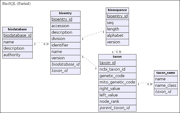
After understanding the schema, let us look into some queries in the next section.
BioSQL Queries
Let us delve into some SQL queries to better understand how the data are organized and the tables are related to each other. Before proceeding, let us open the database using the below command and set some formatting commands −
> sqlite3 orchid.db
SQLite version 3.25.2 2018-09-25 19:08:10
Enter ".help" for usage hints.
sqlite> .header on
sqlite> .mode columns
.header and .mode are formatting options to better visualize the data. You can also use any SQLite editor to run the query.
List the virtual sequence database available in the system as given below −
select
   *
from
   biodatabase;
*** Result ***
sqlite> .width 15 15 15 15
sqlite> select * from biodatabase;
biodatabase_id       name        authority       description
---------------  --------------- --------------- ---------------
1                   orchid
sqlite>
Here, we have only one database, orchid.
List the entries (top 3) available in the database orchid with the below given code
select
   be.*,
   bd.name
from
   bioentry be
   inner join
      biodatabase bd
      on bd.biodatabase_id = be.biodatabase_id
where
   bd.name = 'orchid' Limit 1,
   3;
*** Result ***
sqlite> .width 15 15 10 10 10 10 10 50 10 10
sqlite> select be.*, bd.name from bioentry be inner join biodatabase bd on
bd.biodatabase_id = be.biodatabase_id where bd.name = 'orchid' Limit 1,3;
bioentry_id biodatabase_id taxon_id name accession identifier division description version name
--------------- --------------- ---------- ---------- ---------- ---------- ----------
---------- ---------- ----------- ---------- --------- ---------- ----------
2                   1               19       Z78532     Z78532    2765657     PLN
C.californicum  5.8S rRNA  gene    and      ITS1    and   ITS2 DN  1
orchid
3         1         20          Z78531          Z78531         2765656        PLN
C.fasciculatum  5.8S rRNA  gene    and      ITS1    and   ITS2 DN  1
orchid
4         1         21          Z78530          Z78530         2765655        PLN
C.margaritaceum 5.8S rRNA  gene    and      ITS1    and   ITS2  D  1
orchid
sqlite>
List the sequence details associated with an entry (accession − Z78530, name − C. fasciculatum 5.8S rRNA gene and ITS1 and ITS2 DNA) with the given code −
select
   substr(cast(bs.seq as varchar), 0, 10) || '...' as seq,
   bs.length,
   be.accession,
   be.description,
   bd.name
from
   biosequence bs
   inner join
      bioentry be
      on be.bioentry_id = bs.bioentry_id
   inner join
      biodatabase bd
      on bd.biodatabase_id = be.biodatabase_id
where
   bd.name = 'orchid'
   and be.accession = 'Z78532';
*** Result ***

sqlite> .width 15 5 10 50 10
sqlite> select substr(cast(bs.seq as varchar), 0, 10) || '...' as seq,
bs.length, be.accession, be.description, bd.name from biosequence bs inner
join bioentry be on be.bioentry_id = bs.bioentry_id inner join biodatabase bd
on bd.biodatabase_id = be.biodatabase_id where bd.name = 'orchid' and
be.accession = 'Z78532';
seq           length    accession   description  name
------------ ---------- ---------- ------------ ------------ ---------- ---------- -----------------
CGTAACAAG...    753    Z78532    C.californicum 5.8S rRNA gene and ITS1 and ITS2 DNA orchid
sqlite>
Get the complete sequence associated with an entry (accession − Z78530, name − C. fasciculatum 5.8S rRNA gene and ITS1 and ITS2 DNA) using the below code −
select
   bs.seq
from
   biosequence bs
   inner join
      bioentry be
      on be.bioentry_id = bs.bioentry_id
   inner join
      biodatabase bd
      on bd.biodatabase_id = be.biodatabase_id
where
   bd.name = 'orchid'
   and be.accession = 'Z78532';
*** Result ***

sqlite> .width 1000
sqlite> select bs.seq from biosequence bs inner join bioentry be on
be.bioentry_id = bs.bioentry_id inner join biodatabase bd on bd.biodatabase_id =
be.biodatabase_id where bd.name = 'orchid' and be.accession = 'Z78532';
seq
----------------------------------------------------------------------------------------
----------------------------
CGTAACAAGGTTTCCGTAGGTGAACCTGCGGAAGGATCATTGTTGAGACAACAGAATATATGATCGAGTGAATCT
GGAGGACCTGTGGTAACTCAGCTCGTCGTGGCACTGCTTTTGTCGTGACCCTGCTTTGTTGTTGGGCCTCC
TCAAGAGCTTTCATGGCAGGTTTGAACTTTAGTACGGTGCAGTTTGCGCCAAGTCATATAAAGCATCACTGATGAATGACATTATTGT
CAGAAAAAATCAGAGGGGCAGTATGCTACTGAGCATGCCAGTGAATTTTTATGACTCTCGCAACGGATATCTTGGCTC
TAACATCGATGAAGAACGCAG
sqlite>
List taxon associated with bio database, orchid
select distinct
   tn.name
from
   biodatabase d
   inner join
      bioentry e
      on e.biodatabase_id = d.biodatabase_id
   inner join
      taxon t
      on t.taxon_id = e.taxon_id
   inner join
      taxon_name tn
      on tn.taxon_id = t.taxon_id
where
   d.name = 'orchid' limit 10;
*** Result ***

sqlite> select distinct tn.name from biodatabase d inner join bioentry e on
e.biodatabase_id = d.biodatabase_id inner join taxon t on t.taxon_id =
e.taxon_id inner join taxon_name tn on tn.taxon_id = t.taxon_id where d.name =
'orchid' limit 10;
name
------------------------------
Cypripedium irapeanum
Cypripedium californicum
Cypripedium fasciculatum
Cypripedium margaritaceum
Cypripedium lichiangense
Cypripedium yatabeanum
Cypripedium guttatum
Cypripedium acaule
pink lady's slipper
Cypripedium formosanum
sqlite>
Load Data into BioSQL Database
Let us learn how to load sequence data into the BioSQL database in this chapter. We already have the code to load data into the database in previous section and the code is as follows −
from Bio import SeqIO
from BioSQL import BioSeqDatabase
import os

server = BioSeqDatabase.open_database(driver = 'sqlite3', db = "orchid.db")
DBSCHEMA = "biosqldb-sqlite.sql"
SQL_FILE = os.path.join(os.getcwd(), DBSCHEMA)

server.load_database_sql(SQL_FILE)
server.commit()

db = server.new_database("orchid")
count = db.load(SeqIO.parse("orchid.gbk", "gb"), True) server.commit()
server.close()
We will have a deeper look at every line of the code and its purpose −
Line 1 − Loads the SeqIO module.
Line 2 − Loads the BioSeqDatabase module. This module provides all the functionality to interact with BioSQL database.
Line 3 − Loads os module.
Line 5 − open_database opens the specified database (db) with the configured driver (driver) and returns a handle to the BioSQL database (server). Biopython supports sqlite, mysql, postgresql and oracle databases.
Line 6-10 − load_database_sql method loads the sql from the external file and executes it. commit method commits the transaction. We can skip this step because we already created the database with schema.
Line 12 − new_database methods creates new virtual database, orchid and returns a handle db to execute the command against the orchid database.
Line 13 − load method loads the sequence entries (iterable SeqRecord) into the orchid database. SqlIO.parse parses the GenBank database and returns all the sequences in it as iterable SeqRecord. Second parameter (True) of the load method instructs it to fetch the taxonomy details of the sequence data from NCBI blast website, if it is not already available in the system.
Line 14 − commit commits the transaction.
Line 15 − close closes the database connection and destroys the server handle.
Fetch the Sequence Data
Let us fetch a sequence with identifier, 2765658 from the orchid database as below −
from BioSQL import BioSeqDatabase

server = BioSeqDatabase.open_database(driver = 'sqlite3', db = "orchid.db")

db = server["orchid"]
seq_record = db.lookup(gi = 2765658)
print(seq_record.id, seq_record.description[:50] + "...")
print("Sequence length %i," % len(seq_record.seq))
Here, server["orchid"] returns the handle to fetch data from virtual databaseorchid. lookup method provides an option to select sequences based on criteria and we have selected the sequence with identifier, 2765658. lookup returns the sequence information as SeqRecordobject. Since, we already know how to work with SeqRecord`, it is easy to get data from it.
Remove a Database
Removing a database is as simple as calling remove_database method with proper database name and then committing it as specified below −
from BioSQL import BioSeqDatabase
server = BioSeqDatabase.open_database(driver = 'sqlite3', db = "orchid.db")
server.remove_database("orchids")
server.commit()
Biopython - Population Genetics
Population genetics plays an important role in evolution theory. It analyses the genetic difference between species as well as two or more individuals within the same species.
Biopython provides Bio.PopGen module for population genetics and mainly supports `GenePop, a popular genetics package developed by Michel Raymond and Francois Rousset.
A simple parser
Let us write a simple application to parse the GenePop format and understand the concept.
Download the genePop file provided by Biopython team in the link given below −https://raw.githubusercontent.com/biopython/biopython/master/Tests/PopGen/c3line.gen
Load the GenePop module using the below code snippet −
>>> from Bio.PopGen import GenePop
Parse the file using GenePop.read method as below −
>>> record = GenePop.read(open("c3line.gen"))
Show the loci and population information as given below −
>>> record.loci_list
['136255903', '136257048', '136257636']
>>> record.pop_list
['4', 'b3', '5']
>>> record.populations
[[('1', [(3, 3), (4, 4), (2, 2)]), ('2', [(3, 3), (3, 4), (2, 2)]),
   ('3', [(3, 3), (4, 4), (2, 2)]), ('4', [(3, 3), (4, 3), (None, None)])],
[('b1', [(None, None), (4, 4), (2, 2)]), ('b2', [(None, None), (4, 4), (2, 2)]),
   ('b3', [(None, None), (4, 4), (2, 2)])],
[('1', [(3, 3), (4, 4), (2, 2)]), ('2', [(3, 3), (1, 4), (2, 2)]),
   ('3', [(3, 2), (1, 1), (2, 2)]), ('4',
   [(None, None), (4, 4), (2, 2)]), ('5', [(3, 3), (4, 4), (2, 2)])]]
>>>
Here, there are three loci available in the file and three sets of population: First population has 4 records, second population has 3 records and third population has 5 records. record.populations shows all sets of population with alleles data for each locus.
Manipulate the GenePop file
Biopython provides options to remove locus and population data.
Remove a population set by position,
>>> record.remove_population(0)
>>> record.populations
[[('b1', [(None, None), (4, 4), (2, 2)]),
   ('b2', [(None, None), (4, 4), (2, 2)]),
   ('b3', [(None, None), (4, 4), (2, 2)])],
   [('1', [(3, 3), (4, 4), (2, 2)]),
   ('2', [(3, 3), (1, 4), (2, 2)]),
   ('3', [(3, 2), (1, 1), (2, 2)]),
   ('4', [(None, None), (4, 4), (2, 2)]),
   ('5', [(3, 3), (4, 4), (2, 2)])]]
>>>
Remove a locus by position
>>> record.remove_locus_by_position(0)
>>> record.loci_list
['136257048', '136257636']
>>> record.populations
[[('b1', [(4, 4), (2, 2)]), ('b2', [(4, 4), (2, 2)]), ('b3', [(4, 4), (2, 2)])],
   [('1', [(4, 4), (2, 2)]), ('2', [(1, 4), (2, 2)]),
   ('3', [(1, 1), (2, 2)]), ('4', [(4, 4), (2, 2)]), ('5', [(4, 4), (2, 2)])]]
>>>
Remove a locus by name
>>> record.remove_locus_by_name('136257636')
>>> record.loci_list
['136257048']
>>> record.populations
[[('b1', [(4, 4)]), ('b2', [(4, 4)]), ('b3', [(4, 4)])],
   [('1', [(4, 4)]), ('2', [(1, 4)]),
   ('3', [(1, 1)]), ('4', [(4, 4)]), ('5', [(4, 4)])]]
>>>
Biopython - Genome Analysis
A genome is complete set of DNA, including all of its genes. Genome analysis refers to the study of individual genes and their roles in inheritance.
Genome Diagram
Genome diagram represents the genetic information as charts. Biopython uses Bio.Graphics.GenomeDiagram module to represent GenomeDiagram. The GenomeDiagram module requires ReportLab to be installed.
Steps for creating a diagram
The process of creating a diagram generally follows the below simple pattern −
Create a FeatureSet for each separate set of features you want to display, and add Bio.SeqFeature objects to them.
Create a GraphSet for each graph you want to display, and add graph data to them.
Create a Track for each track you want on the diagram, and add GraphSets and FeatureSets to the tracks you require.
Create a Diagram, and add the Tracks to it.
Tell the Diagram to draw the image.
Write the image to a file.
example.gbk
Let us take an example of input GenBank file −
LOCUS       Z78533                   740 bp    DNA     linear   PLN 30-NOV-2006
DEFINITION  C.irapeanum 5.8S rRNA gene and ITS1 and ITS2 DNA.
ACCESSION   Z78533
VERSION     Z78533.1  GI:2765658
KEYWORDS    5.8S ribosomal RNA; 5.8S rRNA gene; internal transcribed spacer;
            ITS1; ITS2.
SOURCE      Cypripedium irapeanum
  ORGANISM  Cypripedium irapeanum
            Eukaryota; Viridiplantae; Streptophyta; Embryophyta; Tracheophyta;
            Spermatophyta; Magnoliophyta; Liliopsida; Asparagales; Orchidaceae;
            Cypripedioideae; Cypripedium.
REFERENCE   1
  AUTHORS   Cox,A.V., Pridgeon,A.M., Albert,V.A. and Chase,M.W.
  TITLE     Phylogenetics of the slipper orchids (Cypripedioideae:
            Orchidaceae): nuclear rDNA ITS sequences
  JOURNAL   Unpublished
REFERENCE   2  (bases 1 to 740)
  AUTHORS   Cox,A.V.
  TITLE     Direct Submission
  JOURNAL   Submitted (19-AUG-1996) Cox A.V., Royal Botanic Gardens, Kew,
            Richmond, Surrey TW9 3AB, UK
FEATURES             Location/Qualifiers
     source          1..740
                     /organism="Cypripedium irapeanum"
                     /mol_type="genomic DNA"
                     /db_xref="taxon:49711"
     misc_feature    1..380
                     /note="internal transcribed spacer 1"
     gene            381..550
                     /gene="5.8S rRNA"
     rRNA            381..550
                     /gene="5.8S rRNA"
                     /product="5.8S ribosomal RNA"
     misc_feature    551..740
                     /note="internal transcribed spacer 2"
ORIGIN
        1 cgtaacaagg tttccgtagg tgaacctgcg gaaggatcat tgatgagacc gtggaataaa
       61 cgatcgagtg aatccggagg accggtgtac tcagctcacc gggggcattg ctcccgtggt
      121 gaccctgatt tgttgttggg ccgcctcggg agcgtccatg gcgggtttga acctctagcc
      181 cggcgcagtt tgggcgccaa gccatatgaa agcatcaccg gcgaatggca ttgtcttccc
      241 caaaacccgg agcggcggcg tgctgtcgcg tgcccaatga attttgatga ctctcgcaaa
      301 cgggaatctt ggctctttgc atcggatgga aggacgcagc gaaatgcgat aagtggtgtg
      361 aattgcaaga tcccgtgaac catcgagtct tttgaacgca agttgcgccc gaggccatca
      421 ggctaagggc acgcctgctt gggcgtcgcg cttcgtctct ctcctgccaa tgcttgcccg
      481 gcatacagcc aggccggcgt ggtgcggatg tgaaagattg gccccttgtg cctaggtgcg
      541 gcgggtccaa gagctggtgt tttgatggcc cggaacccgg caagaggtgg acggatgctg
      601 gcagcagctg ccgtgcgaat cccccatgtt gtcgtgcttg tcggacaggc aggagaaccc
      661 ttccgaaccc caatggaggg cggttgaccg ccattcggat gtgaccccag gtcaggcggg
      721 ggcacccgct gagtttacgc
//
Install reportLab using pip if not installed.
(myenv) D:\biopython\myenv>pip3 install reportlab
Collecting reportlab
  Obtaining dependency information for reportlab from https://files.pythonhosted.org/packages/0e/ee/5f7a31ab05cf817e0cc70ae6df51a1a4fda188c899790a3131a24dd78d18/reportlab-4.4.6-py3-none-any.whl.metadata
  Downloading reportlab-4.4.6-py3-none-any.whl.metadata (1.7 kB)
Collecting pillow>=9.0.0 (from reportlab)
  Obtaining dependency information for pillow>=9.0.0 from https://files.pythonhosted.org/packages/a2/0b/d87733741526541c909bbf159e338dcace4f982daac6e5a8d6be225ca32d/pillow-12.0.0-cp312-cp312-win_amd64.whl.metadata
  Downloading pillow-12.0.0-cp312-cp312-win_amd64.whl.metadata (9.0 kB)
Collecting charset-normalizer (from reportlab)
  Obtaining dependency information for charset-normalizer from https://files.pythonhosted.org/packages/3d/2d/1e5ed9dd3b3803994c155cd9aacb60c82c331bad84daf75bcb9c91b3295e/charset_normalizer-3.4.4-cp312-cp312-win_amd64.whl.metadata
  Using cached charset_normalizer-3.4.4-cp312-cp312-win_amd64.whl.metadata (38 kB)
Downloading reportlab-4.4.6-py3-none-any.whl (2.0 MB)
   ━━━━━━━━━━━━━━━━━━━━━━━━━━━━━━━━━━━━━━━━ 2.0/2.0 MB 6.9 MB/s eta 0:00:00
Downloading pillow-12.0.0-cp312-cp312-win_amd64.whl (7.0 MB)
   ━━━━━━━━━━━━━━━━━━━━━━━━━━━━━━━━━━━━━━━━ 7.0/7.0 MB 5.3 MB/s eta 0:00:00
Using cached charset_normalizer-3.4.4-cp312-cp312-win_amd64.whl (107 kB)
Installing collected packages: pillow, charset-normalizer, reportlab
Successfully installed charset-normalizer-3.4.4 pillow-12.0.0 reportlab-4.4.6
We shall import all the modules first as shown below −
>>> from reportlab.lib import colors
>>> from reportlab.lib.units import cm
>>> from Bio.Graphics import GenomeDiagram
Now, import SeqIO module to read data −
>>> from Bio import SeqIO
record = SeqIO.read("example.gbk", "genbank")
Here, the record reads the sequence from genbank file.
Now, create an empty diagram to add track and feature set −
>>> diagram = GenomeDiagram.Diagram(
   "Yersinia pestis biovar Microtus plasmid pPCP1")
>>> track = diagram.new_track(1, name="Annotated Features")
>>> feature = track.new_set()
Let us draw a diagram for the above input records −
>>> diagram.draw(
   format = "linear", orientation = "landscape", pagesize = 'A4',
   ... fragments = 4, start = 0, end = len(record))
>>> diagram.write("orchid.pdf", "PDF")
>>> diagram.write("orchid.eps", "EPS")
>>> diagram.write("orchid.svg", "SVG")
After executing the above command, you could see the following image saved in your Biopython directory.
genome.svg
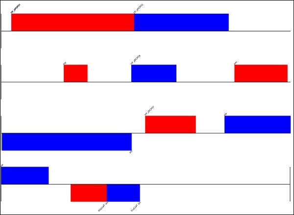
You can also draw the image in circular format by making the below changes −
>>> diagram.draw(
   format = "circular", circular = True, pagesize = (20*cm,20*cm),
   ... start = 0, end = len(record), circle_core = 0.7)
>>> diagram.write("circular.pdf", "PDF")
Chromosomes Overview
DNA molecule is packaged into thread-like structures called chromosomes. Each chromosome is made up of DNA tightly coiled many times around proteins called histones that support its structure.
Chromosomes are not visible in the cells nucleus not even under a microscope when the cell is not dividing. However, the DNA that makes up chromosomes becomes more tightly packed during cell division and is then visible under a microscope.
In humans, each cell normally contains 23 pairs of chromosomes, for a total of 46. Twenty-two of these pairs, called autosomes, look the same in both males and females. The 23rd pair, the sex chromosomes, differ between males and females. Females have two copies of the X chromosome, while males have one X and one Y chromosome.
Biopython - Phenotype Microarray
Phenotype is defined as an observable character or trait exhibited by an organism against a particular chemical or environment. Phenotype microarray simultaneously measures the reaction of an organism against a larger number of chemicals & environment and analyses the data to understand the gene mutation, gene characters, etc.
Biopython provides an excellent module, Bio.Phenotype to analyze phenotypic data. Let us learn how to parse, interpolate, extract and analyze the phenotype microarray data in this chapter.
Parsing
Phenotype microarray data can be in two formats: CSV and JSON. Biopython supports both the formats. Biopython parser parses the phenotype microarray data and returns as a collection of PlateRecord objects. Each PlateRecord object contains a collection of WellRecord objects. Each WellRecord object holds data in 8 rows and 12 columns format. The eight rows are represented by A to H and 12 columns are represented by 01 to 12. For example, 4th row and 6th column are represented by D06.
Let us understand the format and the concept of parsing with the following example −
Step 1 − Download the Plates.csv file provided by Biopython team − https://raw.githubusercontent.com/biopython/biopython/master/Doc/examples/Plates.csv
Step 2 − Load the phenotpe module as below −
>>> from Bio import phenotype
Step 3 − Invoke phenotype.parse method passing the data file and format option (pm-csv). It returns the iterable PlateRecord as below,
>>> plates = list(phenotype.parse('Plates.csv', "pm-csv"))
>>> plates
[PlateRecord('WellRecord['A01'], WellRecord['A02'], WellRecord['A03'], ..., WellRecord['H12']'),
PlateRecord('WellRecord['A01'], WellRecord['A02'], WellRecord['A03'], ..., WellRecord['H12']'),
PlateRecord('WellRecord['A01'], WellRecord['A02'], WellRecord['A03'], ..., WellRecord['H12']'),
PlateRecord('WellRecord['A01'], WellRecord['A02'],WellRecord['A03'], ..., WellRecord['H12']')]
>>>
Step 4 − Access the first plate from the list as below −
>>> plate = plates[0]
>>> plate
PlateRecord('WellRecord['A01'], WellRecord['A02'], WellRecord['A03'], ...,WellRecord['H12']')
>>>
Step 5 − As discussed earlier, a plate contains 8 rows each having 12 items. WellRecord can be access in two ways as specified below −
>>> well = plate["A04"]
>>> well
WellRecord('(0.0, 0.0), (0.25, 0.0), (0.5, 0.0), (0.75, 0.0), (1.0, 0.0), ..., (71.75, 37.0)')
>>> well = plate[0, 4]
>>> well
WellRecord('(0.0, 0.0), (0.25, 0.0), (0.5, 0.0), (0.75, 0.0), (1.0, 0.0), ..., (71.75, 388.0)')
>>>
Step 6 − Each well will have series of measurement at different time points and it can be accessed using for loop as specified below −
>>> for v1, v2 in well:
...  print(v1, v2)
...
0.0 0.0
0.25 0.0
0.5 0.0
0.75 0.0
1.0 0.0
...
71.25 388.0
71.5 388.0
71.75 388.0
>>>
Interpolation
Interpolation gives more insight into the data. Biopython provides methods to interpolate WellRecord data to get information for intermediate time points. The syntax is similar to list indexing and so, easy to learn.
To get the data at 20.1 hours, just pass as index values as specified below −
>>> well[20.10]
69.40000000000003
>>>
We can pass start time point and end time point as well as specified below −
>>> well[20:30]
[67.0, 84.0, 102.0, 119.0, 135.0, 147.0, 158.0, 168.0, 179.0, 186.0]
>>>
The above command interpolate data from 20 hour to 30 hours with 1 hour interval. By default, the interval is 1 hour and we can change it to any value. For example, let us give 15 minutes (0.25 hour) interval as specified below −
>>> well[20:21:0.25]
[67.0, 73.0, 75.0, 81.0]
>>>
Analyze and Extract
Biopython provides a method fit to analyze the WellRecord data using Gompertz, Logistic and Richards sigmoid functions. By default, the fit method uses Gompertz function. We need to call the fit method of the WellRecord object to get the task done. The coding is as follows −
>>> well.fit()
Traceback (most recent call last):
...
Bio.MissingPythonDependencyError: Install scipy to extract curve parameters.
>>> well.model
>>> getattr(well, 'min')
0.0
>>> getattr(well, 'max')
388.0
>>> getattr(well, 'average_height')
205.42708333333334
>>>
Biopython depends on scipy module to do advanced analysis. It will calculate min, max and average_height details without using scipy module.
Biopython - Plotting
This chapter explains about how to plot sequences. Before moving to this topic, let us understand the basics of plotting.
Plotting
Matplotlib is a Python plotting library which produces quality figures in a variety of formats. We can create different types of plots like line chart, histograms, bar chart, pie chart, scatter chart, etc.
pyLab is a module that belongs to the matplotlib which combines the numerical module numpy with the graphical plotting module pyplot.Biopython uses pylab module for plotting sequences. To do this, we need to import the below code −
>>>import pylab
Before importing, we need to install the matplotlib package using pip command with the command given below −
(myenv) D:\biopython\myenv>pip3 install matplotlib
Sample Input File - plot.fasta
Create a sample file named plot.fasta in your Biopython directory and add the following changes −
>gi|2765658|emb|Z78533.1|CIZ78533 C.irapeanum 5.8S rRNA gene and ITS1 and ITS2 DNA
CGTAACAAGGTTTCCGTAGGTGAACCTGCGGAAGGATCATTGATGAGACCGTGGAATAAACGATCGAGTG
AATCCGGAGGACCGGTGTACTCAGCTCACCGGGGGCATTGCTCCCGTGGTGACCCTGATTTGTTGTTGGG
CCGCCTCGGGAGCGTCCATGGCGGGTTTGAACCTCTAGCCCGGCGCAGTTTGGGCGCCAAGCCATATGAA
AGCATCACCGGCGAATGGCATTGTCTTCCCCAAAACCCGGAGCGGCGGCGTGCTGTCGCGTGCCCAATGA
ATTTTGATGACTCTCGCAAACGGGAATCTTGGCTCTTTGCATCGGATGGAAGGACGCAGCGAAATGCGAT
AAGTGGTGTGAATTGCAAGATCCCGTGAACCATCGAGTCTTTTGAACGCAAGTTGCGCCCGAGGCCATCA
GGCTAAGGGCACGCCTGCTTGGGCGTCGCGCTTCGTCTCTCTCCTGCCAATGCTTGCCCGGCATACAGCC
AGGCCGGCGTGGTGCGGATGTGAAAGATTGGCCCCTTGTGCCTAGGTGCGGCGGGTCCAAGAGCTGGTGT
TTTGATGGCCCGGAACCCGGCAAGAGGTGGACGGATGCTGGCAGCAGCTGCCGTGCGAATCCCCCATGTT
GTCGTGCTTGTCGGACAGGCAGGAGAACCCTTCCGAACCCCAATGGAGGGCGGTTGACCGCCATTCGGAT
GTGACCCCAGGTCAGGCGGGGGCACCCGCTGAGTTTACGC

>gi|2765657|emb|Z78532.1|CCZ78532 C.californicum 5.8S rRNA gene and ITS1 and ITS2 DNA
CGTAACAAGGTTTCCGTAGGTGAACCTGCGGAAGGATCATTGTTGAGACAACAGAATATATGATCGAGTG
AATCTGGAGGACCTGTGGTAACTCAGCTCGTCGTGGCACTGCTTTTGTCGTGACCCTGCTTTGTTGTTGG
GCCTCCTCAAGAGCTTTCATGGCAGGTTTGAACTTTAGTACGGTGCAGTTTGCGCCAAGTCATATAAAGC
ATCACTGATGAATGACATTATTGTCAGAAAAAATCAGAGGGGCAGTATGCTACTGAGCATGCCAGTGAAT
TTTTATGACTCTCGCAACGGATATCTTGGCTCTAACATCGATGAAGAACGCAGCTAAATGCGATAAGTGG
TGTGAATTGCAGAATCCCGTGAACCATCGAGTCTTTGAACGCAAGTTGCGCTCGAGGCCATCAGGCTAAG
GGCACGCCTGCCTGGGCGTCGTGTGTTGCGTCTCTCCTACCAATGCTTGCTTGGCATATCGCTAAGCTGG
CATTATACGGATGTGAATGATTGGCCCCTTGTGCCTAGGTGCGGTGGGTCTAAGGATTGTTGCTTTGATG
GGTAGGAATGTGGCACGAGGTGGAGAATGCTAACAGTCATAAGGCTGCTATTTGAATCCCCCATGTTGTT
GTATTTTTTCGAACCTACACAAGAACCTAATTGAACCCCAATGGAGCTAAAATAACCATTGGGCAGTTGA
TTTCCATTCAGATGCGACCCCAGGTCAGGCGGGGCCACCCGCTGAGTTGAGGC

>gi|2765656|emb|Z78531.1|CFZ78531 C.fasciculatum 5.8S rRNA gene and ITS1 and ITS2 DNA
CGTAACAAGGTTTCCGTAGGTGAACCTGCGGAAGGATCATTGTTGAGACAGCAGAACATACGATCGAGTG
AATCCGGAGGACCCGTGGTTACACGGCTCACCGTGGCTTTGCTCTCGTGGTGAACCCGGTTTGCGACCGG
GCCGCCTCGGGAACTTTCATGGCGGGTTTGAACGTCTAGCGCGGCGCAGTTTGCGCCAAGTCATATGGAG
CGTCACCGATGGATGGCATTTTTGTCAAGAAAAACTCGGAGGGGCGGCGTCTGTTGCGCGTGCCAATGAA
TTTATGACGACTCTCGGCAACGGGATATCTGGCTCTTGCATCGATGAAGAACGCAGCGAAATGCGATAAG
TGGTGTGAATTGCAGAATCCCGCGAACCATCGAGTCTTTGAACGCAAGTTGCGCCCGAGGCCATCAGGCT
AAGGGCACGCCTGCCTGGGCGTCGTGTGCTGCGTCTCTCCTGATAATGCTTGATTGGCATGCGGCTAGTC
TGTCATTGTGAGGACGTGAAAGATTGGCCCCTTGCGCCTAGGTGCGGCGGGTCTAAGCATCGGTGTTCTG
ATGGCCCGGAACTTGGCAGTAGGTGGAGGATGCTGGCAGCCGCAAGGCTGCCGTTCGAATCCCCCGTGTT
GTCGTACTCGTCAGGCCTACAGAAGAACCTGTTTGAACCCCCAGTGGACGCAAAACCGCCCTCGGGCGGT
GATTTCCATTCAGATGCGACCCCAGTCAGGCGGGCCACCCGTGAGTAA

>gi|2765655|emb|Z78530.1|CMZ78530 C.margaritaceum 5.8S rRNA gene and ITS1 and ITS2 DNA
CGTAACAAGGTTTCCGTAGGTGAACCTGCGGAAGGATCATTGTTGAAACAACATAATAAACGATTGAGTG
AATCTGGAGGACTTGTGGTAATTTGGCTCGCTAGGGATATCCTTTTGTGGTGACCATGATTTGTCATTGG
GCCTCATTGAGAGCTTTCATGGCGGGTTTGAACCTCTAGCACGGTCCAGTTTGCACCAAGGTATATAAAG
AATCACCGATGAATGACATTATTGCCCCACACAACGTCGGAGGTGTGGTGTGTTAATGTTCATTCCAATG
AATTTTGATGACTCTCGGCAGACGGATATCTTGACTCTTGCATCGATGAAGAACGCACCGAAATGTGATA
AGTGGTGTGAATTGCAGAATCCCGTGAACCATCGAGTCTTTGAACGCAAGTTGCGCCCGAGGCCATCAGG
CTAAGGGCACGCCTGCCTGGGCGTCGTATGTTTTATCTCTCCTTCCAATGCTTGTCCAGCATATAGCTAG
GCCATCATTGTGTGGATGTGAAAGATTGGCCCCTTGTGCTTAGGTGCGGTGGGTCTAAGGATATGTGTTT
TGATGGTCTGAAACTTGGCAAGAGGTGGAGGATGCTGGCAGCCGCAAGGCTATTGTTTGAATCCCCCATG
TTGTCATGTTTGTTGGGCCTATAGAACAACTTGTTTGGACCCTAATTAAGGCAAAACAATCCTTGGGTGG
TTGATTTCCAATCAGATGCGACCCCAGTCAGGGGGCCACCCCAT

>gi|2765654|emb|Z78529.1|CLZ78529 C.lichiangense 5.8S rRNA gene and ITS1 and ITS2 DNA
ACGGCGAGCTGCCGAAGGACATTGTTGAGACAGCAGAATATACGATTGAGTGAATCTGGAGGACTTGTGG
TTATTTGGCTCGCTAGGGATTTCCTTTTGTGGTGACCATGATTTGTCATTGGGCCTCATTGAGAGCTTTC
ATGGCGGGTTTGAACCTCTAGCACGGTGCAGTTTGCACCAAGGTATATAAAGAATCACCGATGAATGACA
TTATTGTCAAAAAAGTCGGAGGTGTGGTGTGTTATTGGTCATGCCAATGAATTGTTGATGACTCTCGCCG
AGGGATATCTTGGCTCTTGCATCGATGAAGAATCCCACCGAAATGTGATAAGTGGTGTGAATTGCAGAAT
CCCGTGAACCATCGAGTCTTTGAACGCAAGTTGCGCCCGAGGCCATCAGGCTAAGGGCACGCCTGCCTGG
GCGTCGTATGTTTTATCTCTCCTTCCAATGCTTGTCCAGCATATAGCTAGGCCATCATTGTGTGGATGTG
AAAGATTGGCCCCTTGTGCTTAGGTGCGGTGGGTCTAAGGATATGTGTTTTGATGGTCTGAAACTTGGCA
AGAGGTGGAGGATGCTGGCAGCCGCAAGGCTATTGTTTGAATCCCCCATGTTGTCATATTTGTTGGGCCT
ATAGAACAACTTGTTTGGACCCTAATTAAGGCAAAACAATCCTTGGGTGGTTGATTTCCAATCAGATGCG
ACCCCAGTCAGCGGGCCACCAGCTGAGCTAAAA
Line Plot
Now, let us create a simple line plot for the above fasta file.
Step 1 − Import SeqIO module to read fasta file.
>>> from Bio import SeqIO
Step 2 − Parse the input file.
>>> records = [len(rec) for rec in SeqIO.parse("plot.fasta", "fasta")]
>>> len(records)
>>> len(records)
5
>>> max(records)
753
>>> min(records)
733
Step 3 − Let us import pylab module.
>>> import pylab
Step 4 − Configure the line chart by assigning x and y axis labels.
>>> pylab.xlabel("sequence length")
Text(0.5, 0, 'sequence length')

>>> pylab.ylabel("count")
Text(0, 0.5, 'count')
>>>
Step 5 − Configure the line chart by setting grid display.
>>> pylab.grid()
Step 6 − Draw simple line chart by calling plot method and supplying records as input.
>>> pylab.plot(records)
[<matplotlib.lines.Line2D object at 0x000001CDC4BC6D80>]
Step 7 − Finally save the chart using the below command.
>>> pylab.savefig("lines.png")
Result
After executing the above command, you could see the following image saved in your Biopython directory.
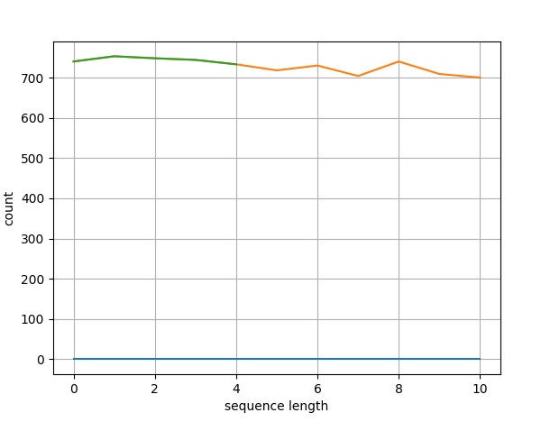
Histogram Chart
A histogram is used for continuous data, where the bins represent ranges of data. Drawing histogram is same as line chart except pylab.plot. Instead, call hist method of pylab module with records and some custum value for bins (5). The complete coding is as follows −
Step 1 − Import SeqIO module to read fasta file.
>>> from Bio import SeqIO
Step 2 − Parse the input file.
>>> records = [len(rec) for rec in SeqIO.parse("plot.fasta", "fasta")]
>>> len(records)
5
>>> max(records)
753
>>> min(records)
733
Step 3 − Let us import pylab module.
>>> import pylab
Step 4 − Configure the line chart by assigning x and y axis labels.
>>> pylab.xlabel("sequence length")
Text(0.5, 0, 'sequence length')

>>> pylab.ylabel("count")
Text(0, 0.5, 'count')
>>>
Step 5 − Configure the line chart by setting grid display.
>>> pylab.grid()
Step 6 − Draw simple line chart by calling plot method and supplying records as input.
>>> pylab.hist(records,bins=5)
array([1., 1., 1., 1., 1.]), array([733., 737., 741., 745., 749., 753.]), <BarContainer object of 5 artists>)
>>>
Step 7 − Finally save the chart using the below command.
>>> pylab.savefig("hist.png")
Result
After executing the above command, you could see the histogram saved in your Biopython directory.
Biopython - Cluster Analysis
In general, Cluster analysis is grouping a set of objects in the same group. This concept is mainly used in data mining, statistical data analysis, machine learning, pattern recognition, image analysis, bioinformatics, etc. It can be achieved by various algorithms to understand how the cluster is widely used in different analysis.
According to Bioinformatics, cluster analysis is mainly used in gene expression data analysis to find groups of genes with similar gene expression.
In this chapter, we will check out important algorithms in Biopython to understand the fundamentals of clustering on a real dataset.
Biopython uses Bio.Cluster module for implementing all the algorithms. It supports the following algorithms −
- Hierarchical Clustering
- K - Clustering
- Self-Organizing Maps
- Principal Component Analysis
Let us have a brief introduction on the above algorithms.
Hierarchical Clustering
Hierarchical clustering is used to link each node by a distance measure to its nearest neighbor and create a cluster. Bio.Cluster node has three attributes: left, right and distance. Let us create a simple cluster as shown below −
>>> from Bio.Cluster import Node
>>> n = Node(1,10)
>>> n.left = 11
>>> n.right = 0
>>> n.distance = 1
>>> print(n)
(11, 0): 1
If you want to construct Tree based clustering, use the below command −
>>> from Bio.Cluster import Tree
>>> n1 = [Node(1, 2, 0.2), Node(0, -1, 0.5)]
>>> n1_tree = Tree(n1)
>>> print(n1_tree)
(1, 2): 0.2
(0, -1): 0.5
>>> print(n1_tree[0])
(1, 2): 0.2
Let us perform hierarchical clustering using Bio.Cluster module.
Consider the distance is defined in an array.
>>> import numpy as np
>>> distance = np.array([[1,2,3],[4,5,6],[3,5,7]])
Now add the distance array in tree cluster.
>>> from Bio.Cluster import treecluster
>>> cluster = treecluster(distance)
>>> print(cluster)
(2, 1): 0.666667
(-1, 0): 9.66667
The above function returns a Tree cluster object. This object contains nodes where the number of items are clustered as rows or columns.
K - Clustering
It is a type of partitioning algorithm and classified into k - means, medians and medoids clustering. Let us understand each of the clustering in brief.
K-means Clustering
This approach is popular in data mining. The goal of this algorithm is to find groups in the data, with the number of groups represented by the variable K.
The algorithm works iteratively to assign each data point to one of the K groups based on the features that are provided. Data points are clustered based on feature similarity.
>>> from Bio.Cluster import kcluster
>>> from numpy import array
>>> data = array([[1, 2], [3, 4], [5, 6]])
>>> clusterid, error,found = kcluster(data)
>>> print(clusterid)
[0 0 1]
>>> print(found)
1
K-medians Clustering
It is another type of clustering algorithm which calculates the mean for each cluster to determine its centroid.
K-medoids Clustering
This approach is based on a given set of items, using the distance matrix and the number of clusters passed by the user.
Consider the distance matrix as defined below −
>>> distance = array([[1,2,3],[4,5,6],[3,5,7]])
We can calculate k-medoids clustering using the below command −
>>> from Bio.Cluster import kmedoids
>>> clusterid, error, found = kmedoids(distance)
>>> print(clusterid)
[0 1 0]
>>> print(found)
1
Let us consider an example.
The kcluster function takes a data matrix as input and not Seq instances. You need to convert your sequences to a matrix and provide that to the kcluster function.
One way of converting the data to a matrix containing numerical elements only is by using the numpy.fromstring function. It basically translates each letter in a sequence to its ASCII counterpart.
This creates a 2D array of encoded sequences that the kcluster function recognized and uses to cluster your sequences.
>>> from Bio.Cluster import kcluster
>>> import numpy as np
>>> sequence = [ 'AGCT','CGTA','AAGT','TCCG']
>>> matrix = np.asarray([np.frombuffer(s.encode('utf-8'), dtype=np.uint8) for s in sequence])
>>> clusterid,error,found = kcluster(matrix)
>>> print(clusterid)
[0 1 1 0]
Self-Organizing Maps
This approach is a type of artificial neural network. It is developed by Kohonen and often called as Kohonen map. It organizes items into clusters based on rectangular topology.
Let us create a simple cluster using the same array distance as shown below −
>>> from Bio.Cluster import somcluster
>>> from numpy import array
>>> data = array([[1, 2], [3, 4], [5, 6]])
>>> clusterid,map = somcluster(data)
>>> print(map)
[[[-0.93529791  1.06076285]]

 [[ 1.23639554 -0.68653191]]]
>>> print(clusterid)
[[0 0]
 [0 0]
 [1 0]]
Here, clusterid is an array with two columns, where the number of rows is equal to the number of items that were clustered, and data is an array with dimensions either rows or columns.
Principal Component Analysis
Principal Component Analysis is useful to visualize high-dimensional data. It is a method that uses simple matrix operations from linear algebra and statistics to calculate a projection of the original data into the same number or fewer dimensions.
Principal Component Analysis returns a tuple columnmean, coordinates, components, and eigenvalues. Let us look into the basics of this concept.
>>> from numpy import array
>>> from numpy import mean
>>> from numpy import cov
>>> from numpy.linalg import eig

# define a matrix
>>> A = array([[1, 2], [3, 4], [5, 6]])

>>> print(A)
[[1 2]
   [3 4]
   [5 6]]

# calculate the mean of each column
>>> M = mean(A.T, axis = 1)
>>> print(M)
[ 3. 4.]

# center columns by subtracting column means
>>> C = A - M

>>> print(C)
[[-2. -2.]
   [ 0. 0.]
   [ 2. 2.]]

# calculate covariance matrix of centered matrix
>>> V = cov(C.T)

>>> print(V)
[[ 4. 4.]
   [ 4. 4.]]

# eigendecomposition of covariance matrix
>>> values, vectors = eig(V)

>>> print(vectors)
[[ 0.70710678 -0.70710678]
   [ 0.70710678 0.70710678]]

>>> print(values)
[ 8. 0.]
Let us apply the same rectangular matrix data to Bio.Cluster module as defined below −
>>> from Bio.Cluster import pca
>>> from numpy import array
>>> data = array([[1, 2], [3, 4], [5, 6]])
>>> columnmean, coordinates, components, eigenvalues = pca(data)
>>> print(columnmean)
[ 3. 4.]
>>> print(coordinates)
[[-2.82842712  0.        ]
 [ 0.          0.        ]
 [ 2.82842712  0.        ]]
>>> print(components)
[[ 0.70710678 0.70710678]
   [ 0.70710678 -0.70710678]]
>>> print(eigenvalues)
[ 4. 0.]
Biopython - Machine Learning
Bioinformatics is an excellent area to apply machine learning algorithms. Here, we have genetic information of large number of organisms and it is not possible to manually analyze all this information. If proper machine learning algorithm is used, we can extract lot of useful information from these data. Biopython provides useful set of algorithm to do supervised machine learning.
Supervised learning is based on input variable (X) and output variable (Y). It uses an algorithm to learn the mapping function from the input to the output. It is defined below −
Y = f(X)
The main objective of this approach is to approximate the mapping function and when you have new input data (x), you can predict the output variables (Y) for that data.
Logistic Regression Model
Logistic regression is a supervised machine Learning algorithm. It is used to find out the difference between K classes using weighted sum of predictor variables. It computes the probability of an event occurrence and can be used for cancer detection.
Biopython provides Bio.LogisticRegression module to predict variables based on Logistic regression algorithm. Currently, Biopython implements logistic regression algorithm for two classes only (K = 2).
k-Nearest Neighbors
k-Nearest neighbors is also a supervised machine learning algorithm. It works by categorizing the data based on nearest neighbors. Biopython provides Bio.KNN module to predict variables based on k-nearest neighbors algorithm.
Naive Bayes
Naive Bayes classifiers are a collection of classification algorithms based on Bayes Theorem. It is not a single algorithm but a family of algorithms where all of them share a common principle, i.e. every pair of features being classified is independent of each other. Biopython provides Bio.NaiveBayes module to work with Naive Bayes algorithm.
Markov Model
A Markov model is a mathematical system defined as a collection of random variables, that experiences transition from one state to another according to certain probabilistic rules. Biopython provides Bio.MarkovModel and Bio.HMM.MarkovModel modules to work with Markov models.
Biopython - Testing Techniques
Biopython have extensive test script to test the software under different conditions to make sure that the software is bug-free. To run the test script, download the source code of the Biopython and then run the below command −
py run_tests.py
This will run all the test scripts and gives the following output −
Python version: 3.12.1
[GCC 4.2.1 (Apple Inc. build 5666) (dot 3)]
Operating system: posix darwin
test_Ace ... ok
test_Affy ... ok
test_AlignIO ... ok
test_AlignIO_ClustalIO ... ok
test_AlignIO_EmbossIO ... ok
test_AlignIO_FastaIO ... ok
test_AlignIO_MauveIO ... ok
test_AlignIO_PhylipIO ... ok
test_AlignIO_convert ... ok
...........................................
...........................................
We can also run individual test script as specified below −
python test_AlignIO.py
Conclusion
As we have learned, Biopython is one of the important software in the field of bioinformatics. Being written in python (easy to learn and write), It provides extensive functionality to deal with any computation and operation in the field of bioinformatics. It also provides easy and flexible interface to almost all the popular bioinformatics software to exploit the its functionality as well.