- Apache MXNet - Home
- Apache MXNet - Introduction
- Apache MXNet - Installing MXNet
- Apache MXNet - Toolkits and Ecosystem
- Apache MXNet - System Architecture
- Apache MXNet - System Components
- Apache MXNet - Unified Operator API
- Apache MXNet - Distributed Training
- Apache MXNet - Python Packages
- Apache MXNet - NDArray
- Apache MXNet - Gluon
- Apache MXNet - KVStore and Visualization
- Apache MXNet - Python API ndarray
- Apache MXNet - Python API gluon
- Apache MXNet - Python API autograd and initializer
- Apache MXNet - Python API Symbol
- Apache MXNet - Python API Module
- Apache MXNet Useful Resources
- Apache MXNet - Quick Guide
- Apache MXNet - Useful Resources
- Apache MXNet - Discussion
Apache MXNet - Python Packages
In this chapter we will learn about the Python Packages available in Apache MXNet.
Important MXNet Python packages
MXNet has the following important Python packages which we will be discussing one by one −
Autograd (Automatic Differentiation)
NDArray
KVStore
Gluon
Visualization
First let us start with Autograd Python package for Apache MXNet.
Autograd
Autograd stands for automatic differentiation used to backpropagate the gradients from the loss metric back to each of the parameters. Along with backpropagation it uses a dynamic programming approach to efficiently calculate the gradients. It is also called reverse mode automatic differentiation. This technique is very efficient in fan-in situations where, many parameters effect a single loss metric.
What are gradients?
Gradients are the fundamentals to the process of neural network training. They basically tell us how to change the parameters of the network to improve its performance.
As we know that, neural networks (NN) are composed of operators such as sums, product, convolutions, etc. These operators, for their computations, use parameters such as the weights in convolution kernels. We should have to find the optimal values for these parameters and gradients shows us the way and lead us to the solution as well.
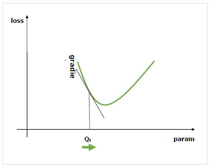
We are interested in the effect of changing a parameter on performance of the network and gradients tell us, how much a given variable increases or decreases when we change a variable it depends on. The performance is usually defined by using a loss metric that we try to minimise. For example, for regression we might try to minimise L2 loss between our predictions and exact value, whereas for classification we might minimise the cross-entropy loss.
Once we calculate the gradient of each parameter with reference to the loss, we can then use an optimiser, such as stochastic gradient descent.
How to calculate gradients?
We have the following options to calculate gradients −
Symbolic Differentiation − The very first option is Symbolic Differentiation, which calculates the formulas for each gradient. The drawback of this method is that, it will quickly lead to incredibly long formulas as the network get deeper and operators get more complex.
Finite Differencing − Another option is, to use finite differencing which try slight differences on each parameter and see how the loss metric responds. The drawback of this method is that, it would be computationally expensive and may have poor numerical precision.
Automatic differentiation − The solution to the drawbacks of the above methods is, to use automatic differentiation to backpropagate the gradients from the loss metric back to each of the parameters. Propagation allows us a dynamic programming approach to efficiently calculate the gradients. This method is also called reverse mode automatic differentiation.
Automatic Differentiation (autograd)
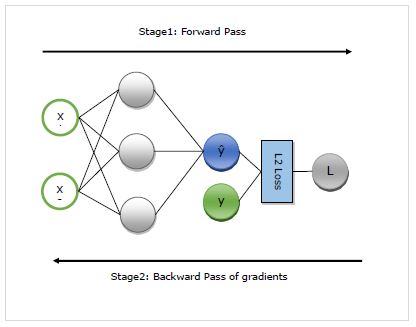
Here, we will understand in detail the working of autograd. It basically works in following two stages −
Stage 1 − This stage is called Forward Pass of training. As name implies, in this stage it creates the record of the operator used by the network to make predictions and calculate the loss metric.
Stage 2 − This stage is called Backward Pass of training. As name implies, in this stage it works backwards through this record. Going backwards, it evaluates the partial derivatives of each operator, all the way back to the network parameter.
Advantages of autograd
Following are the advantages of using Automatic Differentiation (autograd) −
Flexible − Flexibility, that it gives us when defining our network, is one of the huge benefits of using autograd. We can change the operations on every iteration. These are called the dynamic graphs, which are much more complex to implement in frameworks requiring static graph. Autograd, even in such cases, will still be able to backpropagate the gradients correctly.
Automatic − Autograd is automatic, i.e. the complexities of the backpropagation procedure are taken care of by it for you. We just need to specify what gradients we are interested in calculating.
Efficient − Autogard calculates the gradients very efficiently.
Can use native Python control flow operators − We can use the native Python control flow operators such as if condition and while loop. The autograd will still be able to backpropagate the gradients efficiently and correctly.
Using autograd in MXNet Gluon
Here, with the help of an example, we will see how we can use autograd in MXNet Gluon.
Implementation Example
In the following example, we will implement the regression model having two layers. After implementing, we will use autograd to automatically calculate the gradient of the loss with reference to each of the weight parameters −
First import the autogrard and other required packages as follows −
from mxnet import autograd
import mxnet as mx
from mxnet.gluon.nn import HybridSequential, Dense
from mxnet.gluon.loss import L2Loss
Now, we need to define the network as follows −
N_net = HybridSequential()
N_net.add(Dense(units=3))
N_net.add(Dense(units=1))
N_net.initialize()
Now we need to define the loss as follows −
loss_function = L2Loss()
Next, we need to create the dummy data as follows −
x = mx.nd.array([[0.5, 0.9]])
y = mx.nd.array([[1.5]])
Now, we are ready for our first forward pass through the network. We want autograd to record the computational graph so that we can calculate the gradients. For this, we need to run the network code in the scope of autograd.record context as follows −
with autograd.record():
   y_hat = N_net(x)
   loss = loss_function(y_hat, y)
Now, we are ready for the backward pass, which we start by calling the backward method on the quantity of interest. The quatity of interest in our example is loss because we are trying to calculate the gradient of loss with reference to the parameters −
loss.backward()
Now, we have gradients for each parameter of the network, which will be used by the optimiser to update the parameter value for improved performance. Lets check out the gradients of the 1st layer as follows −
N_net[0].weight.grad()
Output
The output is as follows−
[[-0.00470527 -0.00846948]
[-0.03640365 -0.06552657]
[ 0.00800354 0.01440637]]
<NDArray 3x2 @cpu(0)>
Complete implementation example
Given below is the complete implementation example.
from mxnet import autograd
import mxnet as mx
from mxnet.gluon.nn import HybridSequential, Dense
from mxnet.gluon.loss import L2Loss
N_net = HybridSequential()
N_net.add(Dense(units=3))
N_net.add(Dense(units=1))
N_net.initialize()
loss_function = L2Loss()
x = mx.nd.array([[0.5, 0.9]])
y = mx.nd.array([[1.5]])
with autograd.record():
y_hat = N_net(x)
loss = loss_function(y_hat, y)
loss.backward()
N_net[0].weight.grad()