OpenCV Python - Fourier Transform

---

---

The Fourier Transform is used to transform an image from its spatial domain to its frequency domain by decomposing it into its sinus and cosines components.

In case of digital images, a basic gray scale image values usually are between zero and 255. Therefore, the Fourier Transform too needs to be a Discrete Fourier Transform (DFT). It is used to find the frequency domain.

Mathematically, Fourier Transform of a two dimensional image is represented as follows −

$$\mathrm{F(k,l)=\displaystyle\sum\limits_{i=0}^{N-1}\: \displaystyle\sum\limits_{j=0}^{N-1} f(i,j)\:e^{-i2\pi (\frac{ki}{N},\frac{lj}{N})}}$$

If the amplitude varies so fast in a short time, you can say it is a high frequency signal. If it varies slowly, it is a low frequency signal.

In case of images, the amplitude varies drastically at the edge points, or noises. So edges and noises are high frequency contents in an image. If there are no much changes in amplitude, it is a low frequency component.

OpenCV provides the functions cv.dft() and cv.idft() for this purpose.

cv.dft() performs a Discrete Fourier transform of a 1D or 2D floating-point array. The command for the same is as follows −

cv.dft(src, dst, flags)

Here,

• src − Input array that could be real or complex.
• dst − Output array whose size and type depends on the flags.
• flags − Transformation flags, representing a combination of the DftFlags.

cv.idft() calculates the inverse Discrete Fourier Transform of a 1D or 2D array. The command for the same is as follows −

cv.idft(src, dst, flags)

In order to obtain a discrete fourier transform, the input image is converted to np.float32 datatype. The transform obtained is then used to Shift the zero-frequency component to the center of the spectrum, from which magnitude spectrum is calculated.

Example

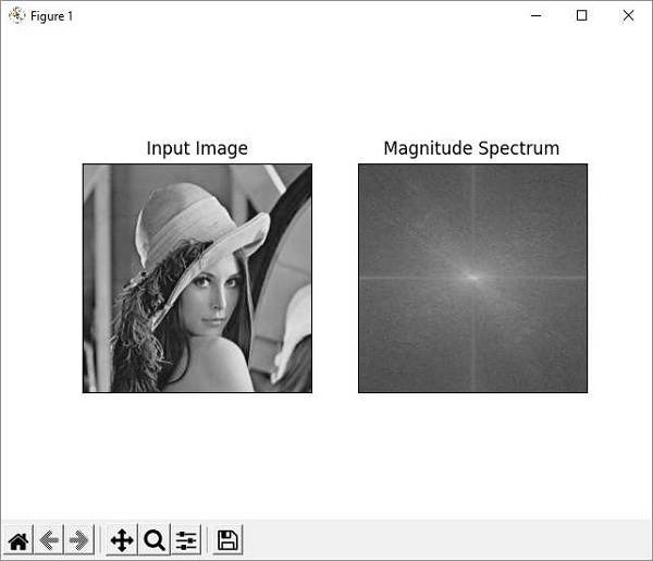
Given below is the program using Matplotlib, we plot the original image and magnitude spectrum −

import numpy as np
import cv2 as cv
from matplotlib import pyplot as plt
img = cv.imread('lena.jpg',0)
dft = cv.dft(np.float32(img),flags = cv.DFT_COMPLEX_OUTPUT)
dft_shift = np.fft.fftshift(dft)
magnitude_spectrum = 20*np.log(cv.magnitude(dft_shift[:,:,0],dft_shift[:,:,1]))
plt.subplot(121),plt.imshow(img, cmap = 'gray')
plt.title('Input Image'), plt.xticks([]), plt.yticks([])
plt.subplot(122),plt.imshow(magnitude_spectrum, cmap = 'gray')
plt.title('Magnitude Spectrum'), plt.xticks([]), plt.yticks([])
plt.show()

Output