- Estimation Techniques - Home
- Estimation Techniques - Overview
- Estimation Techniques - FP
- Estimation Techniques - FP Counting
- Estimation Techniques - Use-case
- Estimation Techniques - Delphi
- Estimation Techniques - Three-point
- Estimation Techniques - PERT
- Estimation Techniques - Analogous
- Estimation Techniques - WBS
- Estimation - Planning Poker
- Estimation Techniques - Testing
Estimation Techniques - Quick Guide
Estimation Techniques - Overview
Estimation is the process of finding an estimate, or approximation, which is a value that can be used for some purpose even if input data may be incomplete, uncertain, or unstable.
Estimation determines how much money, effort, resources, and time it will take to build a specific system or product. Estimation is based on −
- Past Data/Past Experience
- Available Documents/Knowledge
- Assumptions
- Identified Risks
The four basic steps in Software Project Estimation are −
- Estimate the size of the development product.
- Estimate the effort in person-months or person-hours.
- Estimate the schedule in calendar months.
- Estimate the project cost in agreed currency.
Observations on Estimation
Estimation need not be a one-time task in a project. It can take place during −
- Acquiring a Project.
- Planning the Project.
- Execution of the Project as the need arises.
Project scope must be understood before the estimation process begins. It will be helpful to have historical Project Data.
Project metrics can provide a historical perspective and valuable input for generation of quantitative estimates.
Planning requires technical managers and the software team to make an initial commitment as it leads to responsibility and accountability.
Past experience can aid greatly.
Use at least two estimation techniques to arrive at the estimates and reconcile the resulting values. Refer Decomposition Techniques in the next section to learn about reconciling estimates.
Plans should be iterative and allow adjustments as time passes and more details are known.
General Project Estimation Approach
The Project Estimation Approach that is widely used is Decomposition Technique. Decomposition techniques take a divide and conquer approach. Size, Effort and Cost estimation are performed in a stepwise manner by breaking down a Project into major Functions or related Software Engineering Activities.
Step 1 − Understand the scope of the software to be built.
Step 2 − Generate an estimate of the software size.
Start with the statement of scope.
Decompose the software into functions that can each be estimated individually.
Calculate the size of each function.
Derive effort and cost estimates by applying the size values to your baseline productivity metrics.
Combine function estimates to produce an overall estimate for the entire project.
Step 3 − Generate an estimate of the effort and cost. You can arrive at the effort and cost estimates by breaking down a project into related software engineering activities.
Identify the sequence of activities that need to be performed for the project to be completed.
Divide activities into tasks that can be measured.
Estimate the effort (in person hours/days) required to complete each task.
Combine effort estimates of tasks of activity to produce an estimate for the activity.
Obtain cost units (i.e., cost/unit effort) for each activity from the database.
Compute the total effort and cost for each activity.
Combine effort and cost estimates for each activity to produce an overall effort and cost estimate for the entire project.
Step 4 − Reconcile estimates: Compare the resulting values from Step 3 to those obtained from Step 2. If both sets of estimates agree, then your numbers are highly reliable. Otherwise, if widely divergent estimates occur conduct further investigation concerning whether −
The scope of the project is not adequately understood or has been misinterpreted.
The function and/or activity breakdown is not accurate.
Historical data used for the estimation techniques is inappropriate for the application, or obsolete, or has been misapplied.
Step 5 − Determine the cause of divergence and then reconcile the estimates.
Estimation Accuracy
Accuracy is an indication of how close something is to reality. Whenever you generate an estimate, everyone wants to know how close the numbers are to reality. You will want every estimate to be as accurate as possible, given the data you have at the time you generate it. And of course you dont want to present an estimate in a way that inspires a false sense of confidence in the numbers.
Important factors that affect the accuracy of estimates are −
The accuracy of all the estimates input data.
The accuracy of any estimate calculation.
How closely the historical data or industry data used to calibrate the model matches the project you are estimating.
The predictability of your organizations software development process.
The stability of both the product requirements and the environment that supports the software engineering effort.
Whether or not the actual project was carefully planned, monitored and controlled, and no major surprises occurred that caused unexpected delays.
Following are some guidelines for achieving reliable estimates −
- Base estimates on similar projects that have already been completed.
- Use relatively simple decomposition techniques to generate project cost and effort estimates.
- Use one or more empirical estimation models for software cost and effort estimation.
Refer to the section on Estimation Guidelines in this chapter.
To ensure accuracy, you are always advised to estimate using at least two techniques and compare the results.
Estimation Issues
Often, project managers resort to estimating schedules skipping to estimate size. This may be because of the timelines set by the top management or the marketing team. However, whatever the reason, if this is done, then at a later stage it would be difficult to estimate the schedules to accommodate the scope changes.
While estimating, certain assumptions may be made. It is important to note all these assumptions in the estimation sheet, as some still do not document assumptions in estimation sheets.
Even good estimates have inherent assumptions, risks, and uncertainty, and yet they are often treated as though they are accurate.
The best way of expressing estimates is as a range of possible outcomes by saying, for example, that the project will take 5 to 7 months instead of stating it will be complete on a particular date or it will be complete in a fixed no. of months. Beware of committing to a range that is too narrow as that is equivalent to committing to a definite date.
You could also include uncertainty as an accompanying probability value. For example, there is a 90% probability that the project will complete on or before a definite date.
Organizations do not collect accurate project data. Since the accuracy of the estimates depend on the historical data, it would be an issue.
For any project, there is a shortest possible schedule that will allow you to include the required functionality and produce quality output. If there is a schedule constraint by management and/or client, you could negotiate on the scope and functionality to be delivered.
Agree with the client on handling scope creeps to avoid schedule overruns.
Failure in accommodating contingency in the final estimate causes issues. For e.g., meetings, organizational events.
Resource utilization should be considered as less than 80%. This is because the resources would be productive only for 80% of their time. If you assign resources at more than 80% utilization, there is bound to be slippages.
Estimation Guidelines
One should keep the following guidelines in mind while estimating a project −
During estimation, ask other people's experiences. Also, put your own experiences at task.
Assume resources will be productive for only 80 percent of their time. Hence, during estimation take the resource utilization as less than 80%.
Resources working on multiple projects take longer to complete tasks because of the time lost switching between them.
Include management time in any estimate.
Always build in contingency for problem solving, meetings and other unexpected events.
Allow enough time to do a proper project estimate. Rushed estimates are inaccurate, high-risk estimates. For large development projects, the estimation step should really be regarded as a mini project.
Where possible, use documented data from your organizations similar past projects. It will result in the most accurate estimate. If your organization has not kept historical data, now is a good time to start collecting it.
Use developer-based estimates, as the estimates prepared by people other than those who will do the work will be less accurate.
Use several different people to estimate and use several different estimation techniques.
Reconcile the estimates. Observe the convergence or spread among the estimates. Convergence means that you have got a good estimate. Wideband-Delphi technique can be used to gather and discuss estimates using a group of people, the intention being to produce an accurate, unbiased estimate.
Re-estimate the project several times throughout its life cycle.
Estimation Techniques - Function Points
A Function Point (FP) is a unit of measurement to express the amount of business functionality, an information system (as a product) provides to a user. FPs measure software size. They are widely accepted as an industry standard for functional sizing.
For sizing software based on FP, several recognized standards and/or public specifications have come into existence. As of 2013, these are −
ISO Standards
COSMIC − ISO/IEC 19761:2011 Software engineering. A functional size measurement method.
FiSMA − ISO/IEC 29881:2008 Information technology - Software and systems engineering - FiSMA 1.1 functional size measurement method.
IFPUG − ISO/IEC 20926:2009 Software and systems engineering - Software measurement - IFPUG functional size measurement method.
Mark-II − ISO/IEC 20968:2002 Software engineering - Ml II Function Point Analysis - Counting Practices Manual.
NESMA − ISO/IEC 24570:2005 Software engineering - NESMA function size measurement method version 2.1 - Definitions and counting guidelines for the application of Function Point Analysis.
Object Management Group Specification for Automated Function Point
Object Management Group (OMG), an open membership and not-for-profit computer industry standards consortium, has adopted the Automated Function Point (AFP) specification led by the Consortium for IT Software Quality. It provides a standard for automating FP counting according to the guidelines of the International Function Point User Group (IFPUG).
Function Point Analysis (FPA) technique quantifies the functions contained within software in terms that are meaningful to the software users. FPs consider the number of functions being developed based on the requirements specification.
Function Points (FP) Counting is governed by a standard set of rules, processes and guidelines as defined by the International Function Point Users Group (IFPUG). These are published in Counting Practices Manual (CPM).
History of Function Point Analysis
The concept of Function Points was introduced by Alan Albrecht of IBM in 1979. In 1984, Albrecht refined the method. The first Function Point Guidelines were published in 1984. The International Function Point Users Group (IFPUG) is a US-based worldwide organization of Function Point Analysis metric software users. The International Function Point Users Group (IFPUG) is a non-profit, member-governed organization founded in 1986. IFPUG owns Function Point Analysis (FPA) as defined in ISO standard 20296:2009 which specifies the definitions, rules and steps for applying the IFPUG's functional size measurement (FSM) method. IFPUG maintains the Function Point Counting Practices Manual (CPM). CPM 2.0 was released in 1987, and since then there have been several iterations. CPM Release 4.3 was in 2010.
The CPM Release 4.3.1 with incorporated ISO editorial revisions was in 2010. The ISO Standard (IFPUG FSM) - Functional Size Measurement that is a part of CPM 4.3.1 is a technique for measuring software in terms of the functionality it delivers. The CPM is an internationally approved standard under ISO/IEC 14143-1 Information Technology Software Measurement.
Elementary Process (EP)
Elementary Process is the smallest unit of functional user requirement that −
- Is meaningful to the user.
- Constitutes a complete transaction.
- Is self-contained and leaves the business of the application being counted in a consistent state.
Functions
There are two types of functions −
- Data Functions
- Transaction Functions
Data Functions
There are two types of data functions −
- Internal Logical Files
- External Interface Files
Data Functions are made up of internal and external resources that affect the system.
Internal Logical Files
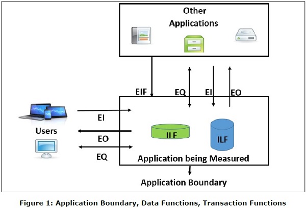
Internal Logical File (ILF) is a user identifiable group of logically related data or control information that resides entirely within the application boundary. The primary intent of an ILF is to hold data maintained through one or more elementary processes of the application being counted. An ILF has the inherent meaning that it is internally maintained, it has some logical structure and it is stored in a file. (Refer Figure 1)
External Interface Files
External Interface File (EIF) is a user identifiable group of logically related data or control information that is used by the application for reference purposes only. The data resides entirely outside the application boundary and is maintained in an ILF by another application. An EIF has the inherent meaning that it is externally maintained, an interface has to be developed to get the data from the file. (Refer Figure 1)
Transaction Functions
There are three types of transaction functions.
- External Inputs
- External Outputs
- External Inquiries
Transaction functions are made up of the processes that are exchanged between the user, the external applications and the application being measured.
External Inputs
External Input (EI) is a transaction function in which Data goes into the application from outside the boundary to inside. This data is coming external to the application.
- Data may come from a data input screen or another application.
- An EI is how an application gets information.
- Data can be either control information or business information.
- Data may be used to maintain one or more Internal Logical Files.
- If the data is control information, it does not have to update an Internal Logical File. (Refer Figure 1)
External Outputs
External Output (EO) is a transaction function in which data comes out of the system. Additionally, an EO may update an ILF. The data creates reports or output files sent to other applications. (Refer Figure 1)
External Inquiries
External Inquiry (EQ) is a transaction function with both input and output components that result in data retrieval. (Refer Figure 1)
Definition of RETs, DETs, FTRs
Record Element Type
A Record Element Type (RET) is the largest user identifiable subgroup of elements within an ILF or an EIF. It is best to look at logical groupings of data to help identify them.
Data Element Type
Data Element Type (DET) is the data subgroup within an FTR. They are unique and user identifiable.
File Type Referenced
File Type Referenced (FTR) is the largest user identifiable subgroup within the EI, EO, or EQ that is referenced to.
The transaction functions EI, EO, EQ are measured by counting FTRs and DETs that they contain following counting rules. Likewise, data functions ILF and EIF are measured by counting DETs and RETs that they contain following counting rules. The measures of transaction functions and data functions are used in FP counting which results in the functional size or function points.
Estimation Techniques - FP Counting Process
FP Counting Process involves the following steps −
Step 1 − Determine the type of count.
Step 2 − Determine the boundary of the count.
Step 3 − Identify each Elementary Process (EP) required by the user.
Step 4 − Determine the unique EPs.
Step 5 − Measure data functions.
Step 6 − Measure transactional functions.
Step 7 − Calculate functional size (unadjusted function point count).
Step 8 − Determine Value Adjustment Factor (VAF).
Step 9 − Calculate adjusted function point count.
Note − General System Characteristics (GSCs) are made optional in CPM 4.3.1 and moved to Appendix. Hence, Step 8 and Step 9 can be skipped.
Step 1: Determine the Type of Count
There are three types of function point counts −
- Development Function Point Count
- Application Function Point Count
- Enhancement Function Point Count
Development Function Point Count
Function points can be counted at all phases of a development project from requirement to implementation stage. This type of count is associated with new development work and may include the prototypes, which may have been required as temporary solution, which supports the conversion effort. This type of count is called a baseline function point count.
Application Function Point Count
Application counts are calculated as the function points delivered, and exclude any conversion effort (prototypes or temporary solutions) and existing functionality that may have existed.
Enhancement Function Point Count
When changes are made to software after production, they are considered as enhancements. To size such enhancement projects, the Function Point Count gets Added, Changed or Deleted in the Application.
Step 2: Determine the Boundary of the Count
The boundary indicates the border between the application being measured and the external applications or the user domain. (Refer Figure 1)
To determine the boundary, understand −
- The purpose of the function point count
- Scope of the application being measured
- How and which applications maintain what data
- The business areas that support the applications
Step 3: Identify Each Elementary Process Required by the User
Compose and/or decompose the functional user requirements into the smallest unit of activity, which satisfies all of the following criteria −
- Is meaningful to the user.
- Constitutes a complete transaction.
- Is self-contained.
- Leaves the business of the application being counted in a consistent state.
For example, the Functional User Requirement − Maintain Employee information can be decomposed into smaller activities such as add employee, change employee, delete employee, and inquire about employee.
Each unit of activity thus identified is an Elementary Process (EP).
Step 4: Determine the Unique Elementary Processes
Comparing two EPs already identified, count them as one EP (same EP) if they −
- Require the same set of DETs.
- Require the same set of FTRs.
- Require the same set of processing logic to complete the EP.
Do not split an EP with multiple forms of processing logic into multiple Eps.
For e.g., if you have identified Add Employee as an EP, it should not be divided into two EPs to account for the fact that an employee may or may not have dependents. The EP is still Add Employee, and there is variation in the processing logic and DETs to account for dependents.
Step 5: Measure Data Functions
Classify each data function as either an ILF or an EIF.
A data function shall be classified as an −
Internal Logical File (ILF), if it is maintained by the application being measured.
External Interface File (EIF) if it is referenced, but not maintained by the application being measured.
ILFs and EIFs can contain business data, control data and rules based data. For example, telephone switching is made of all three types - business data, rule data and control data. Business data is the actual call. Rule data is how the call should be routed through the network, and control data is how the switches communicate with each other.
Consider the following documentation for counting ILFs and EIFs −
- Objectives and constraints for the proposed system.
- Documentation regarding the current system, if such a system exists.
- Documentation of the users perceived objectives, problems and needs.
- Data models.
Step 5.1: Count the DETs for Each Data Function
Apply the following rules to count DETs for ILF/EIF −
Count a DET for each unique user identifiable, non-repeated field maintained in or retrieved from the ILF or EIF through the execution of an EP.
Count only those DETs being used by the application that is measured when two or more applications maintain and/or reference the same data function.
Count a DET for each attribute required by the user to establish a relationship with another ILF or EIF.
Review related attributes to determine if they are grouped and counted as a single DET or whether they are counted as multiple DETs. Grouping will depend on how the EPs use the attributes within the application.
Step 5.2: Count the RETs for Each Data Function
Apply the following rules to count RETs for ILF/EIF −
- Count one RET for each data function.
- Count one additional RET for each of the following additional logical sub-groups of DETs.
- Associative entity with non-key attributes.
- Sub-type (other than the first sub-type).
- Attributive entity, in a relationship other than mandatory 1:1.
Step 5.3: Determine the Functional Complexity for Each Data Function
| RETS | Data Element Types (DETs) | ||
|---|---|---|---|
| 1-19 | 20-50 | >50 | |
| 1 | L | L | A |
| 2 to 5 | L | A | H |
| >5 | A | H | H |
Functional Complexity: L = Low; A = Average; H = High
Step 5.4: Measure the Functional Size for Each Data Function
| Functional Complexity | FP Count for ILF | FP Count for EIF |
|---|---|---|
| Low | 7 | 5 |
| Average | 10 | 7 |
| High | 15 | 10 |
Step 6: Measure Transactional Functions
To measure transactional functions following are the necessary steps −
Step 6.1: Classify each Transactional Function
Transactional functions should be classified as an External Input, External Output or an External Inquiry.
External Input
External Input (EI) is an Elementary Process that processes data or control information that comes from outside the boundary. The primary intent of an EI is to maintain one or more ILFs and/or to alter the behavior of the system.
All of the following rules must be applied −
The data or control information is received from outside the application boundary.
At least one ILF is maintained if the data entering the boundary is not control information that alters the behavior of the system.
For the identified EP, one of the three statements must apply −
Processing logic is unique from processing logic performed by other EIs for the application.
The set of data elements identified is different from the sets identified for other EIs in the application.
ILFs or EIFs referenced are different from the files referenced by the other EIs in the application.
External Output
External Output (EO) is an Elementary Process that sends data or control information outside the applications boundary. EO includes additional processing beyond that of an external inquiry.
The primary intent of an EO is to present information to a user through processing logic other than or in addition to the retrieval of data or control information.
The processing logic must −
- Contain at least one mathematical formula or calculation.
- Create derived data.
- Maintain one or more ILFs.
- Alter the behavior of the system.
All of the following rules must be applied −
- Sends data or control information external to the applications boundary.
- For the identified EP, one of the three statements must apply −
- Processing logic is unique from the processing logic performed by other EOs for the application.
- The set of data elements identified are different from other EOs in the application.
- ILFs or EIFs referenced are different from files referenced by other EOs in the application.
Additionally, one of the following rules must apply −
- The processing logic contains at least one mathematical formula or calculation.
- The processing logic maintains at least one ILF.
- The processing logic alters the behavior of the system.
External Inquiry
External Inquiry (EQ) is an Elementary Process that sends data or control information outside the boundary. The primary intent of an EQ is to present information to the user through the retrieval of data or control information.
The processing logic contains no mathematical formula or calculations, and creates no derived data. No ILF is maintained during the processing, nor is the behavior of the system altered.
All of the following rules must be applied −
- Sends data or control information external to the applications boundary.
- For the identified EP, one of the three statements must apply −
- Processing logic is unique from the processing logic performed by other EQs for the application.
- The set of data elements identified are different from other EQs in the application.
- The ILFs or EIFs referenced are different from the files referenced by other EQs in the application.
Additionally, all of the following rules must apply −
- The processing logic retrieves data or control information from an ILF or EIF.
- The processing logic does not contain mathematical formula or calculation.
- The processing logic does not alter the behavior of the system.
- The processing logic does not maintain an ILF.
Step 6.2: Count the DETs for Each Transactional Function
Apply the following Rules to count DETs for EIs −
Review everything that crosses (enters and/or exits) the boundary.
Count one DET for each unique user identifiable, non-repeated attribute that crosses (enters and/or exits) the boundary during the processing of the transactional function.
Count only one DET per transactional function for the ability to send an application response message, even if there are multiple messages.
Count only one DET per transactional function for the ability to initiate action(s) even if there are multiple means to do so.
Do not count the following items as DETs −
Attributes generated within the boundary by a transactional function and saved to an ILF without exiting the boundary.
Literals such as report titles, screen or panel identifiers, column headings and attribute titles.
Application generated stamps such as date and time attributes.
Paging variables, page numbers and positioning information, for e.g., Rows 37 to 54 of 211.
Navigation aids such as the ability to navigate within a list using previous, next, first, last and their graphical equivalents.
Apply the following rules to count DETs for EOs/EQs −
Review everything that crosses (enters and/or exits) the boundary.
Count one DET for each unique user identifiable, non-repeated attribute that crosses (enters and/or exits) the boundary during the processing of the transactional function.
Count only one DET per transactional function for the ability to send an application response message, even if there are multiple messages.
Count only one DET per transactional function for the ability to initiate action(s) even if there are multiple means to do so.
Do not count the following items as DETs −
Attributes generated within the boundary without crossing the boundary.
Literals such as report titles, screen or panel identifiers, column headings and attribute titles.
Application generated stamps such as date and time attributes.
Paging variables, page numbers and positioning information, for e.g., Rows 37 to 54 of 211.
Navigation aids such as the ability to navigate within a list using previous, next, first, last and their graphical equivalents.
Step 6.3: Count the FTRs for Each Transactional Function
Apply the following rules to count FTRs for EIs −
- Count a FTR for each ILF maintained.
- Count a FTR for each ILF or EIF read during the processing of the EI.
- Count only one FTR for each ILF that is both maintained and read.
Apply the following rule to count FTRs for EO/EQs −
- Count a FTR for each ILF or EIF read during the processing of EP.
Additionally, apply the following rules to count FTRs for EOs −
- Count a FTR for each ILF maintained during the processing of EP.
- Count only one FTR for each ILF that is both maintained and read by EP.
Step 6.4: Determine the Functional Complexity for Each Transactional Function
| FTRs | Data Element Types (DETs) | ||
|---|---|---|---|
| 1-4 | 5-15 | >=16 | |
| 0-1 | L | L | A |
| 2 | L | A | H |
| >=3 | A | H | H |
Functional Complexity: L = Low; A = Average; H = High
Determine the functional complexity for each EO/EQ, with an exception that EQ must have a minimum of 1 FTR −
EQ must have a minimum of 1 FTR FTRs |
Data Element Types (DETs) | ||
|---|---|---|---|
| 1-4 | 5-15 | >=16 | |
| 0-1 | L | L | A |
| 2 | L | A | H |
| >=3 | A | H | H |
Functional Complexity: L = Low; A = Average; H = High
Step 6.5: Measure the Functional Size for Each Transactional Function
Measure the functional size for each EI from its functional complexity.
| Complexity | FP Count |
|---|---|
| Low | 3 |
| Average | 4 |
| High | 6 |
Measure the functional size for each EO/EQ from its functional complexity.
| Complexity | FP Count for EO | FP Count for EQ |
|---|---|---|
| Low | 4 | 3 |
| Average | 5 | 4 |
| High | 6 | 6 |
Step 7: Calculate Functional Size (Unadjusted Function Point Count)
To calculate the functional size, one should follow the steps given below −
Step 7.1
Recollect what you have found in Step 1. Determine the type of count.
Step 7.2
Calculate the functional size or function point count based on the type.
- For development function point count, go to Step 7.3.
- For application function point count, go to Step 7.4.
- For enhancement function point count, go to Step 7.5.
Step 7.3
Development Function Point Count consists of two components of functionality −
Application functionality included in the user requirements for the project.
Conversion functionality included in the user requirements for the project. Conversion functionality consists of functions provided only at installation to convert data and/or provide other user-specified conversion requirements, such as special conversion reports. For e.g. an existing application may be replaced with a new system.
DFP = ADD + CFP
Where,
DFP = Development Function Point Count
ADD = Size of functions delivered to the user by the development project
CFP = Size of the conversion functionality
ADD = FP Count (ILFs) + FP Count (EIFs) + FP Count (EIs) + FP Count (EOs) + FP Count (EQs)
CFP = FP Count (ILFs) + FP Count (EIFs) + FP Count (EIs) + FP Count (EOs) + FP Count (EQs)
Step 7.4
Calculate the Application Function Point Count
AFP = ADD
Where,
AFP = Application Function Point Count
ADD = Size of functions delivered to the user by the development project (excluding the size of any conversion functionality), or the functionality that exists whenever the application is counted.
ADD = FP Count (ILFs) + FP Count (EIFs) + FP Count (EIs) + FP Count (EOs) + FP Count (EQs)
Step 7.5
Enhancement Function Point Count considers the following four components of functionality −
- Functionality that is added to the application.
- Functionality that is modified in the Application.
- Conversion functionality.
- Functionality that is deleted from the application.
EFP = ADD + CHGA + CFP + DEL
Where,
EFP = Enhancement Function Point Count
ADD = Size of functions being added by the enhancement project
CHGA = Size of functions being changed by the enhancement project
CFP = Size of the conversion functionality
DEL = Size of functions being deleted by the enhancement project
ADD = FP Count (ILFs) + FP Count (EIFs) + FP Count (EIs) + FP Count (EOs) + FP Count (EQs)
CHGA = FP Count (ILFs) + FP Count (EIFs) + FP Count (EIs) + FP Count (EOs) + FP Count (EQs)
CFP = FP Count (ILFs) + FP Count (EIFs) + FP Count (EIs) + FP Count (EOs) + FP Count (EQs)
DEL = FP Count (ILFs) + FP Count (EIFs) + FP COUNT (EIs) + FP Count (EOs) + FP Count (EQs)
Step 8: Determine the Value Adjustment Factor
GSCs are made optional in CPM 4.3.1 and moved to Appendix. Hence, Step 8 and Step 9 can be skipped.
The Value Adjustment Factor (VAF) is based on 14 GSCs that rate the general functionality of the application being counted. GSCs are user business constraints independent of technology. Each characteristic has associated descriptions to determine the degree of influence.
| General System Characteristic | Brief Description |
|---|---|
| Data Communications | How many communication facilities are there to aid in the transfer or exchange of information with the application or system? |
| Distributed Data Processing | How are distributed data and processing functions handled? |
| Performance | Did the user require response time or throughput? |
| Heavily Used Configuration | How heavily used is the current hardware platform where the application will be executed? |
| Transaction Rate | How frequently are transactions executed daily, weekly, monthly, etc.? |
| On-Line Data Entry | What percentage of the information is entered online? |
| End-user Efficiency | Was the application designed for end-user efficiency? |
| Online Update | How many ILFs are updated by online transaction? |
| Complex Processing | Does the application have extensive logical or mathematical processing? |
| Reusability | Was the application developed to meet one or many users needs? |
| Installation Ease | How difficult is conversion and installation? |
| Operational Ease | How effective and/or automated are start-up, back-up, and recovery procedures? |
| Multiple Sites | Was the application specifically designed, developed, and supported to be installed at multiple sites for multiple organizations? |
| Facilitate Change | Was the application specifically designed, developed, and supported to facilitate change? |
The degree of influence range is on a scale of zero to five, from no influence to strong influence.
| Rating | Degree of Influence |
|---|---|
| 0 | Not present, or no influence |
| 1 | Incidental influence |
| 2 | Moderate influence |
| 3 | Average influence |
| 4 | Significant influence |
| 5 | Strong influence throughout |
Determine the degree of influence for each of the 14 GSCs.
The sum of the values of the 14 GSCs thus obtained is termed as Total Degree of Influence (TDI).
TDI = ∑14 Degrees of Influence
Next, calculate Value Adjustment Factor (VAF) as
VAF = (TDI × 0.01) + 0.65
Each GSC can vary from 0 to 5, TDI can vary from (0 × 14) to (5 × 14), i.e. 0 (when all GSCs are low) to 70 (when all GSCs are high) i.e. 0 ≤ TDI ≤ 70. Hence, VAF can vary in the range from 0.65 (when all GSCs are low) to 1.35 (when all GSCs are high), i.e., 0.65 ≤ VAF ≤ 1.35.
Step 9: Calculate Adjusted Function Point Count
As per the FPA approach that uses the VAF (CPM versions before V4.3.1), this is determined by,
Adjusted FP Count = Unadjusted FP Count × VAF
Where, unadjusted FP count is the functional size that you have calculated in Step 7.
As the VAF can vary from 0.65 to 1.35, the VAF exerts an influence of ±35% on the final adjusted FP count.
Benefits of Function Points
Function points are useful −
In measuring the size of the solution instead of the size of the problem.
As requirements are the only thing needed for function points count.
As it is independent of technology.
As it is independent of programming languages.
In estimating testing projects.
In estimating overall project costs, schedule and effort.
In contract negotiations as it provides a method of easier communication with business groups.
As it quantifies and assigns a value to the actual uses, interfaces, and purposes of the functions in the software.
In creating ratios with other metrics such as hours, cost, headcount, duration, and other application metrics.
FP Repositories
International Software Benchmarking Standards Group (ISBSG) grows and maintains two repositories for IT data.
- Development and Enhancement Projects
- Maintenance and Support Applications
There are more than 6,000 projects in the Development and Enhancement Projects repository.
Data is delivered in Microsoft Excel format, making it easier for further analysis that you wish to do with it, or you can even use the data for some other purpose.
ISBSG repository license can be purchased from − https://www.isbsg.org/product/corporate-subscription/
ISBSG offers 10% discount for IFPUG members for online purchases when the discount code IFPUGMembers is used.
ISBSG Software Project Data Release updates can be found at: https://ifpug.org/event/isbsg-project-and-application-data
COSMIC and IFPUG collaborated to produce a Glossary of terms for software Non-functional and Project Requirements. It can be downloaded from − cosmic-sizing.org
Estimation Techniques - Use Case Points
A Use-Case is a series of related interactions between a user and a system that enables the user to achieve a goal.
Use-Cases are a way to capture functional requirements of a system. The user of the system is referred to as an Actor. Use-Cases are fundamentally in text form.
Use-Case Points Definition
Use-Case Points (UCP) is a software estimation technique used to measure the software size with use cases. The concept of UCP is similar to FPs.
The number of UCPs in a project is based on the following −
- The number and complexity of the use cases in the system.
- The number and complexity of the actors on the system.
Various non-functional requirements (such as portability, performance, maintainability) that are not written as use cases.
The environment in which the project will be developed (such as the language, the teams motivation, etc.)
Estimation with UCPs requires all use cases to be written with a goal and at approximately the same level, giving the same amount of detail. Hence, before estimation, the project team should ensure they have written their use cases with defined goals and at detailed level. Use case is normally completed within a single session and after the goal is achieved, the user may go on to some other activity.
History of Use-Case Points
The Use-Case Point estimation method was introduced by Gustav Karner in 1993. The work was later licensed by Rational Software that merged into IBM.
Use-Case Points Counting Process
The Use-Case Points counting process has the following steps −
- Calculate unadjusted UCPs
- Adjust for technical complexity
- Adjust for environmental complexity
- Calculate adjusted UCPs
Step 1: Calculate Unadjusted Use-Case Points.
You calculate Unadjusted Use-Case Points first, by the following steps −
- Determine Unadjusted Use-Case Weight
- Determine Unadjusted Actor Weight
- Calculate Unadjusted Use-Case Points
Step 1.1 − Determine Unadjusted Use-Case Weight.
Step 1.1.1 − Find the number of transactions in each Use-Case.
If the Use-Cases are written with User Goal Levels, a transaction is equivalent to a step in the Use-Case. Find the number of transactions by counting the steps in the Use-Case.
Step 1.1.2 − Classify each Use-Case as Simple, Average or Complex based on the number of transactions in the Use-Case. Also, assign Use-Case Weight as shown in the following table −
| Use-Case Complexity | Number of Transactions | Use-Case Weight |
|---|---|---|
| Simple | ≤3 | 5 |
| Average | 4 to 7 | 10 |
| Complex | >7 | 15 |
Step 1.1.3 − Repeat for each Use-Case and get all the Use-Case Weights. Unadjusted Use-Case Weight (UUCW) is the sum of all the Use-Case Weights.
Step 1.1.4 − Find Unadjusted Use-Case Weight (UUCW) using the following table −
| Use-Case Complexity | Use-Case Weight | Number of Use-Cases | Product |
|---|---|---|---|
| Simple | 5 | NSUC | 5 × NSUC |
| Average | 10 | NAUC | 10 × NAUC |
| Complex | 15 | NCUC | 15 × NCUC |
| Unadjusted Use-Case Weight (UUCW) | 5 × NSUC + 10 × NAUC + 15 × NCUC | ||
Where,
NSUC is the no. of Simple Use-Cases.
NAUC is the no. of Average Use-Cases.
NCUC is the no. of Complex Use-Cases.
Step 1.2 − Determine Unadjusted Actor Weight.
An Actor in a Use-Case might be a person, another program, etc. Some actors, such as a system with defined API, have very simple needs and increase the complexity of a Use-Case only slightly.
Some actors, such as a system interacting through a protocol have more needs and increase the complexity of a Use-Case to a certain extent.
Other Actors, such as a user interacting through GUI have a significant impact on the complexity of a Use-Case. Based on these differences, you can classify actors as Simple, Average and Complex.
Step 1.2.1 − Classify Actors as Simple, Average and Complex and assign Actor Weights as shown in the following table −
| Actor Complexity | Example | Actor Weight |
|---|---|---|
| Simple | A System with defined API | 1 |
| Average | A System interacting through a Protocol | 2 |
| Complex | A User interacting through GUI | 3 |
Step 1.2.2 − Repeat for each Actor and get all the Actor Weights. Unadjusted Actor Weight (UAW) is the sum of all the Actor Weights.
Step 1.2.3 − Find Unadjusted Actor Weight (UAW) using the following table −
| Actor Complexity | Actor Weight | Number of Actors | Product |
|---|---|---|---|
| Simple | 1 | NSA | 1 × NSA |
| Average | 2 | NAA | 2 × NAA |
| Complex | 3 | NCA | 3 × NCA |
| Unadjusted Actor Weight (UAW) | 1 × NSA + 2 × NAA + 3 × NCA | ||
Where,
NSA is the no. of Simple Actors.
NAA is the no. of Average Actors.
NCA is the no. of Complex Actors.
Step 1.3 − Calculate Unadjusted Use-Case Points.
The Unadjusted Use-Case Weight (UUCW) and the Unadjusted Actor Weight (UAW) together give the unadjusted size of the system, referred to as Unadjusted Use-Case Points.
Unadjusted Use-Case Points (UUCP) = UUCW + UAW
The next steps are to adjust the Unadjusted Use-Case Points (UUCP) for Technical Complexity and Environmental Complexity.
Step 2: Adjust For Technical Complexity
Step 2.1 − Consider the 13 Factors that contribute to the impact of the Technical Complexity of a project on Use-Case Points and their corresponding Weights as given in the following table −
| Factor | Description | Weight |
|---|---|---|
| T1 | Distributed System | 2.0 |
| T2 | Response time or throughput performance objectives | 1.0 |
| T3 | End user efficiency | 1.0 |
| T4 | Complex internal processing | 1.0 |
| T5 | Code must be reusable | 1.0 |
| T6 | Easy to install | .5 |
| T7 | Easy to use | .5 |
| T8 | Portable | 2.0 |
| T9 | Easy to change | 1.0 |
| T10 | Concurrent | 1.0 |
| T11 | Includes special security objectives | 1.0 |
| T12 | Provides direct access for third parties | 1.0 |
| T13 | Special user training facilities are required | 1.0 |
Many of these factors represent the projects nonfunctional requirements.
Step 2.2 − For each of the 13 Factors, assess the project and rate from 0 (irrelevant) to 5 (very important).
Step 2.3 − Calculate the Impact of the Factor from Impact Weight of the Factor and the Rated Value for the project as
Impact of the Factor = Impact Weight × Rated Value
Step (2.4) − Calculate the sum of Impact of all the Factors. This gives the Total Technical Factor (TFactor) as given in table below −
| Factor | Description | Weight (W) | Rated Value (0 to 5) (RV) | Impact (I = W × RV) |
|---|---|---|---|---|
| T1 | Distributed System | 2.0 | ||
| T2 | Response time or throughput performance objectives | 1.0 | ||
| T3 | End user efficiency | 1.0 | ||
| T4 | Complex internal processing | 1.0 | ||
| T5 | Code must be reusable | 1.0 | ||
| T6 | Easy to install | .5 | ||
| T7 | Easy to use | .5 | ||
| T8 | Portable | 2.0 | ||
| T9 | Easy to change | 1.0 | ||
| T10 | Concurrent | 1.0 | ||
| T11 | Includes special security objectives | 1.0 | ||
| T12 | Provides direct access for third parties | 1.0 | ||
| T13 | Special user training facilities are required | 1.0 | ||
| Total Technical Factor (TFactor) | ||||
Step 2.5 − Calculate the Technical Complexity Factor (TCF) as −
TCF = 0.6 + (0.01 × TFactor)
Step 3: Adjust For Environmental Complexity
Step 3.1 − Consider the 8 Environmental Factors that could affect the project execution and their corresponding Weights as given in the following table −
| Factor | Description | Weight |
|---|---|---|
| F1 | Familiar with the project model that is used | 1.5 |
| F2 | Application experience | .5 |
| F3 | Object-oriented experience | 1.0 |
| F4 | Lead analyst capability | .5 |
| F5 | Motivation | 1.0 |
| F6 | Stable requirements | 2.0 |
| F7 | Part-time staff | -1.0 |
| F8 | Difficult programming language | -1.0 |
Step 3.2 − For each of the 8 Factors, assess the project and rate from 0 (irrelevant) to 5 (very important).
Step 3.3 − Calculate the Impact of the Factor from Impact Weight of the Factor and the Rated Value for the project as
Impact of the Factor = Impact Weight × Rated Value
Step 3.4 − Calculate the sum of Impact of all the Factors. This gives the Total Environment Factor (EFactor) as given in the following table −
| Factor | Description | Weight (W) | Rated Value (0 to 5) (RV) | Impact (I = W × RV) |
|---|---|---|---|---|
| F1 | Familiar with the project model that is used | 1.5 | ||
| F2 | Application experience | .5 | ||
| F3 | Object-oriented experience | 1.0 | ||
| F4 | Lead analyst capability | .5 | ||
| F5 | Motivation | 1.0 | ||
| F6 | Stable requirements | 2.0 | ||
| F7 | Part-time staff | -1.0 | ||
| F8 | Difficult programming language | -1.0 | ||
| Total Environment Factor (EFactor) | ||||
Step 3.5 − Calculate the Environmental Factor (EF) as −
1.4 + (-0.03 × EFactor)
Step 4: Calculate Adjusted Use-Case Points (UCP)
Calculate Adjusted Use-Case Points (UCP) as −
UCP = UUCP × TCF × EF
Advantages and Disadvantages of Use-Case Points
Advantages of Use-Case Points
UCPs are based on use cases and can be measured very early in the project life cycle.
UCP (size estimate) will be independent of the size, skill, and experience of the team that implements the project.
UCP based estimates are found to be close to actuals when estimation is performed by experienced people.
UCP is easy to use and does not call for additional analysis.
Use cases are being used vastly as a method of choice to describe requirements. In such cases, UCP is the best suitable estimation technique.
Disadvantages of Use-Case Points
UCP can be used only when requirements are written in the form of use cases.
Dependent on goal-oriented, well-written use cases. If the use cases are not well or uniformly structured, the resulting UCP may not be accurate.
Technical and environmental factors have a high impact on UCP. Care needs to be taken while assigning values to the technical and environmental factors.
UCP is useful for initial estimate of overall project size but they are much less useful in driving the iteration-to-iteration work of a team.
Estimation Techniques - Wideband Delphi
Delphi Method is a structured communication technique, originally developed as a systematic, interactive forecasting method which relies on a panel of experts. The experts answer questionnaires in two or more rounds. After each round, a facilitator provides an anonymous summary of the experts forecasts from the previous round with the reasons for their judgments. Experts are then encouraged to revise their earlier answers in light of the replies of other members of the panel.
It is believed that during this process the range of answers will decrease and the group will converge towards the "correct" answer. Finally, the process is stopped after a predefined stop criterion (e.g. number of rounds, achievement of consensus, and stability of results) and the mean or median scores of the final rounds determine the results.
Delphi Method was developed in the 1950-1960s at the RAND Corporation.
Wideband Delphi Technique
In the 1970s, Barry Boehm and John A. Farquhar originated the Wideband Variant of the Delphi Method. The term "wideband" is used because, compared to the Delphi Method, the Wideband Delphi Technique involved greater interaction and more communication between the participants.
In Wideband Delphi Technique, the estimation team comprise the project manager, moderator, experts, and representatives from the development team, constituting a 3-7 member team. There are two meetings −
- Kickoff Meeting
- Estimation Meeting
Wideband Delphi Technique Steps
Step 1 − Choose the Estimation team and a moderator.
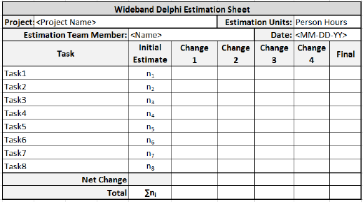
Step 2 − The moderator conducts the kickoff meeting, in which the team is presented with the problem specification and a high level task list, any assumptions or project constraints. The team discusses on the problem and estimation issues, if any. They also decide on the units of estimation. The moderator guides the entire discussion, monitors time and after the kickoff meeting, prepares a structured document containing problem specification, high level task list, assumptions, and the units of estimation that are decided. He then forwards copies of this document for the next step.
Step 3 − Each Estimation team member then individually generates a detailed WBS, estimates each task in the WBS, and documents the assumptions made.
Step 4 − The moderator calls the Estimation team for the Estimation meeting. If any of the Estimation team members respond saying that the estimates are not ready, the moderator gives more time and resends the Meeting Invite.
Step 5 − The entire Estimation team assembles for the estimation meeting.
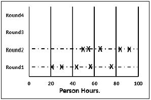
Step 5.1 − At the beginning of the Estimation meeting, the moderator collects the initial estimates from each of the team members.
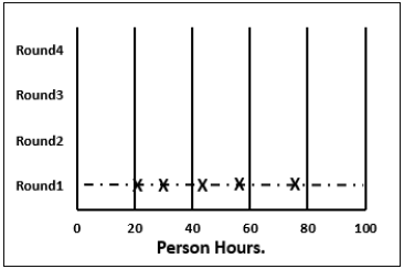
Step 5.2 − He then plots a chart on the whiteboard. He plots each members total project estimate as an X on the Round 1 line, without disclosing the corresponding names. The Estimation team gets an idea of the range of estimates, which initially may be large.
Step 5.3 − Each team member reads aloud the detailed task list that he/she made, identifying any assumptions made and raising any questions or issues. The task estimates are not disclosed.
The individual detailed task lists contribute to a more complete task list when combined.
Step 5.4 − The team then discusses any doubt/problem they have about the tasks they have arrived at, assumptions made, and estimation issues.
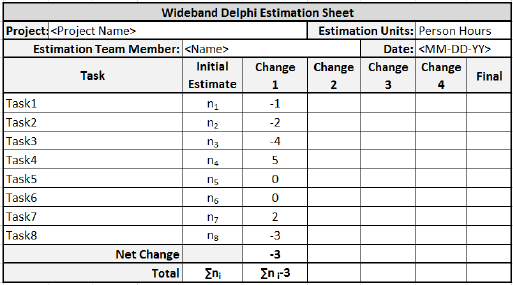
Step 5.5 − Each team member then revisits his/her task list and assumptions, and makes changes if necessary. The task estimates also may require adjustments based on the discussion, which are noted as +N Hrs. for more effort and N Hrs. for less effort.
The team members then combine the changes in the task estimates to arrive at the total project estimate.
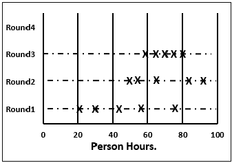
Step 5.6 − The moderator collects the changed estimates from all the team members and plots them on the Round 2 line.
In this round, the range will be narrower compared to the earlier one, as it is more consensus based.
Step 5.7 − The team then discusses the task modifications they have made and the assumptions.
Step 5.8 − Each team member then revisits his/her task list and assumptions, and makes changes if necessary. The task estimates may also require adjustments based on the discussion.
The team members then once again combine the changes in the task estimate to arrive at the total project estimate.
Step 5.9 − The moderator collects the changed estimates from all the members again and plots them on the Round 3 line.
Again, in this round, the range will be narrower compared to the earlier one.
Step 5.10 − Steps 5.7, 5.8, 5.9 are repeated till one of the following criteria is met −
- Results are converged to an acceptably narrow range.
- All team members are unwilling to change their latest estimates.
- The allotted Estimation meeting time is over.
Step 6 − The Project Manager then assembles the results from the Estimation meeting.
Step 6.1 − He compiles the individual task lists and the corresponding estimates into a single master task list.
Step 6.2 − He also combines the individual lists of assumptions.
Step 6.3 − He then reviews the final task list with the Estimation team.
Advantages and Disadvantages of Wideband Delphi Technique
Advantages
- Wideband Delphi Technique is a consensus-based estimation technique for estimating effort.
- Useful when estimating time to do a task.
- Participation of experienced people and they individually estimating would lead to reliable results.
- People who would do the work are making estimates thus making valid estimates.
- Anonymity maintained throughout makes it possible for everyone to express their results confidently.
- A very simple technique.
- Assumptions are documented, discussed and agreed.
Disadvantages
- Management support is required.
- The estimation results may not be what the management wants to hear.
Estimation Techniques - Three Point
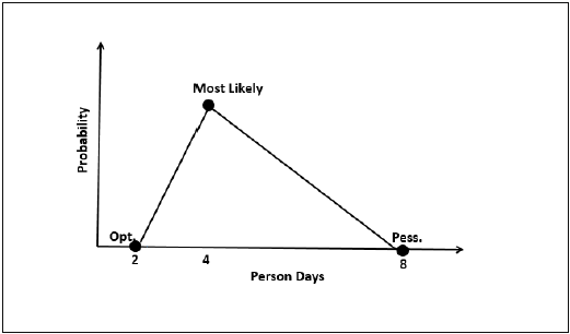
Three-point Estimation looks at three values −
- the most optimistic estimate (O),
- a most likely estimate (M), and
- a pessimistic estimate (least likely estimate (L)).
There has been some confusion regarding Three-point Estimation and PERT in the industry. However, the techniques are different. You will see the differences as you learn the two techniques. Also, at the end of the PERT technique, the differences are collated and presented. If you want to look at them first, you can.
Three-point Estimate (E) is based on the simple average and follows triangular distribution.
E = (O + M + L) / 3
Standard Deviation
In Triangular Distribution,
Mean = (O + M + L) / 3
Standard Deviation = √ [((O − E)2 + (M − E)2 + (L − E)2) / 2]
Three-point Estimation Steps
Step 1 − Arrive at the WBS.
Step 2 − For each task, find three values − most optimistic estimate (O), a most likely estimate (M), and a pessimistic estimate (L).
Step 3 − Calculate the Mean of the three values.
Mean = (O + M + L) / 3
Step 4 − Calculate the Three-point Estimate of the task. Three-point Estimate is the Mean. Hence,
E = Mean = (O + M + L) / 3
Step 5 − Calculate the Standard Deviation of the task.
Standard Deviation (SD) = √ [((O − E)2 + (M − E)2 + (L - E)2)/2]
Step 6 − Repeat Steps 2, 3, 4 for all the Tasks in the WBS.
Step 7 − Calculate the Three-point Estimate of the project.
E (Project) = ∑ E (Task)
Step 8 − Calculate the Standard Deviation of the project.
SD (Project) = √ (∑SD (Task)2)
Convert the Project Estimates to Confidence Levels
The Three-point Estimate (E) and the Standard Deviation (SD) thus calculated are used to convert the project estimates to Confidence Levels.
The conversion is based such that −
- Confidence Level in E +/ SD is approximately 68%.
- Confidence Level in E value +/ 1.645 × SD is approximately 90%.
- Confidence Level in E value +/ 2 × SD is approximately 95%.
- Confidence Level in E value +/ 3 × SD is approximately 99.7%.
Commonly, the 95% Confidence Level, i.e., E Value + 2 × SD, is used for all project and task estimates.
Estimation Techniques - PERT
Project Evaluation and Review Technique (PERT) estimation considers three values: the most optimistic estimate (O), a most likely estimate (M), and a pessimistic estimate (least likely estimate (L)). There has been some confusion regarding Three-point Estimation and PERT in the Industry. However, the techniques are different. You will see the differences as you learn the two techniques. Also, at the end of this chapter, the differences are collated and presented.
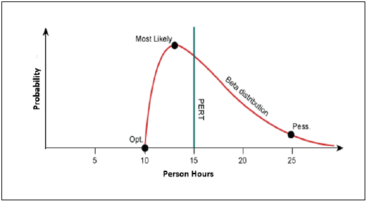
PERT is based on three values − most optimistic estimate (O), a most likely estimate (M), and a pessimistic estimate (least likely estimate (L)). The most-likely estimate is weighted 4 times more than the other two estimates (optimistic and pessimistic).
PERT Estimate (E) is based on the weighted average and follows beta distribution.
E = (O + 4 × M + L)/6
PERT is frequently used along with Critical Path Method (CPM). CPM tells about the tasks that are critical in the project. If there is a delay in these tasks, the project gets delayed.
Standard Deviation
Standard Deviation (SD) measures the variability or uncertainty in the estimate.
In beta distribution,
Mean = (O + 4 × M + L)/6
Standard Deviation (SD) = (L − O)/6
PERT Estimation Steps
Step (1) − Arrive at the WBS.
Step (2) − For each task, find three values most optimistic estimate (O), a most likely estimate (M), and a pessimistic estimate (L).
Step (3) − PERT Mean = (O + 4 × M + L)/6
PERT Mean = (O + 4 × M + L)/3
Step (4) − Calculate the Standard Deviation of the task.
Standard Deviation (SD) = (L − O)/6
Step (6) − Repeat steps 2, 3, 4 for all the tasks in the WBS.
Step (7) − Calculate the PERT estimate of the project.
E (Project) = ∑ E (Task)
Step (8) − Calculate the Standard Deviation of the project.
SD (Project) = √ (SD (Task)2)
Convert the Project Estimates to Confidence Levels
PERT Estimate (E) and Standard Deviation (SD) thus calculated are used to convert the project estimates to confidence levels.
The conversion is based such that
- Confidence level in E +/ SD is approximately 68%.
- Confidence level in E value +/ 1.645 × SD is approximately 90%.
- Confidence level in E value +/ 2 × SD is approximately 95%.
- Confidence level in E value +/ 3 × SD is approximately 99.7%.
Commonly, the 95% confidence level, i.e., E Value + 2 SD, is used for all project and task estimates.
Differences between Three-Point Estimation and PERT
Following are the differences between Three-Point Estimation and PERT −
| Three-Point Estimation | PERT |
|---|---|
| Simple average | Weighted average |
| Follows triangular Distribution | Follows beta Distribution |
| Used for small repetitive projects | Used for large non-repetitive projects, usually R&D projects. Used along with Critical Path Method (CPM) |
E = Mean = (O + M + L)/3 This is simple average |
E = Mean = (O + 4 × M + L)/6 This is weighted average |
| SD = √ [((O − E)2 + (M − E)2 + (L − E)2)/2] | SD = (L − O)/6 |
Estimation Techniques - Analogous
Analogous Estimation uses a similar past project information to estimate the duration or cost of your current project, hence the word, "analogy". You can use analogous estimation when there is limited information regarding your current project.
Quite often, there will be situations when project managers will be asked to give cost and duration estimates for a new project as the executives need decision-making data to decide whether the project is worth doing. Usually, neither the project manager nor anyone else in the organization has ever done a project like the new one but the executives still want accurate cost and duration estimates.
In such cases, analogous estimation is the best solution. It may not be perfect but is accurate as it is based on past data. Analogous estimation is an easy-to-implement technique. The project success rate can be up to 60% as compared to the initial estimates.
Analogous Estimation Definition
Analogous estimation is a technique which uses the values of parameters from historical data as the basis for estimating similar parameter for a future activity. Parameters examples: Scope, cost, and duration. Measures of scale examples − Size, weight, and complexity.
Because the project managers, and possibly the teams experience and judgment are applied to the estimating process, it is considered a combination of historical information and expert judgment.
Analogous Estimation Requirements
For analogous estimation following is the requirement −
- Data from previous and on-going projects
- Work hours per week of each team member
- Costs involved to get the project completed
- Project close to the current project
- In case the current Project is new, and no past project is similar
- Modules from past projects that are similar to those in current project
- Activities from past projects that are similar to those in current project
- Data from these selected ones
- Participation of the project manager and estimation team to ensure experienced judgment on the estimates.
Analogous Estimation Steps
The project manager and team have to collectively do analogous estimation.
Step 1 − Identify the domain of the current project.
Step 2 − Identify the technology of the current project.
Step 3 − Look in the organization database if a similar project data is available. If available, go to Step (4). Otherwise go to Step (6).
Step 4 − Compare the current project with the identified past project data.
Step 5 − Arrive at the duration and cost estimates of the current project. This ends analogous estimation of the project.
Step 6 − Look in the organization database if any past projects have similar modules as those in the current project.
Step 7 − Look in the organization database if any past projects have similar activities as those in the current project.
Step 8 − Collect all those and use expert judgment to arrive at the duration and cost estimates of the current project.
Advantages of Analogous Estimation
Analogous estimation is a better way of estimation in the initial stages of the project when very few details are known.
The technique is simple and time taken for estimation is very less.
Organizations success rate can be expected to be high since the technique is based on the organizations past project data.
Analogous estimation can be used to estimate the effort and duration of individual tasks too. Hence, in WBS when you estimate the tasks, you can use Analogy.
Estimation Techniques - WBS
Work Breakdown Structure (WBS), in Project Management and Systems Engineering, is a deliverable-oriented decomposition of a project into smaller components. WBS is a key project deliverable that organizes the team's work into manageable sections. The Project Management Body of Knowledge (PMBOK) defines WBS as a "deliverable oriented hierarchical decomposition of the work to be executed by the project team."
WBS element may be a product, data, service, or any combination thereof. WBS also provides the necessary framework for detailed cost estimation and control along with providing guidance for schedule development and control.
Representation of WBS
WBS is represented as a hierarchical list of projects work activities. There are two formats of WBS −
- Outline View (Indented Format)
- Tree Structure View (Organizational Chart)
Let us first discuss how to use the outline view for preparing a WBS.
Outline View
The outline view is a very user-friendly layout. It presents a good view of the entire project and allows easy modifications as well. It uses numbers to record the various stages of a project. It looks somewhat similar to the following −
Software Development
Scope
- Determine project scope
- Secure project sponsorship
- Define preliminary resources
- Secure core resources
- Scope complete
Analysis/Software Requirements
- Conduct needs analysis
- Draft preliminary software specifications
- Develop preliminary budget
- Review software specifications/budget with the team
- Incorporate feedback on software specifications
- Develop delivery timeline
- Obtain approvals to proceed (concept, timeline, and budget)
- Secure required resources
- Analysis complete
Design
- Review preliminary software specifications
- Develop functional specifications
- Obtain approval to proceed
- Design complete
Development
- Review functional specifications
- Identify modular/tiered design parameters
- Develop code
- Developer testing (primary debugging)
- Development complete
Testing
- Develop unit test plans using product specifications
- Develop integration test plans using product specifications
Training
- Develop training specifications for end-users
- Identify training delivery methodology (online, classroom, etc.)
- Develop training materials
- Finalize training materials
- Develop training delivery mechanism
- Training materials complete
Deployment
- Determine final deployment strategy
- Develop deployment methodology
- Secure deployment resources
- Train support staff
- Deploy software
- Deployment complete
Let us now take a look at the tree structure view.
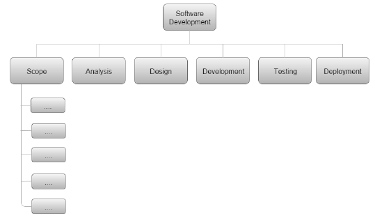
Tree Structure View
The Tree Structure View presents a very easy-to-understand view of the entire project. The following illustration shows how a tree structure view looks like. This type of organizational chart structure can be easily drawn with the features available in MS-Word.
Types of WBS
There are two types of WBS −
Functional WBS − In functional WBS, the system is broken based on the functions in the application to be developed. This is useful in estimating the size of the system.
Activity WBS − In activity WBS, the system is broken based on the activities in the system. The activities are further broken into tasks. This is useful in estimating effort and schedule in the system.
Estimate Size
Step 1 − Start with functional WBS.
Step 2 − Consider the leaf nodes.
Step 3 − Use either Analogy or Wideband Delphi to arrive at the size estimates.
Estimate Effort
Step 1 − Use Wideband Delphi Technique to construct WBS. We suggest that the tasks should not be more than 8 hrs. If a task is of larger duration, split it.
Step 2 − Use Wideband Delphi Technique or Three-point Estimation to arrive at the Effort Estimates for the Tasks.
Scheduling
Once the WBS is ready and the size and effort estimates are known, you are ready for scheduling the tasks.
While scheduling the tasks, certain things should be taken into account −
Precedence − A task that must occur before another is said to have precedence of the other.
Concurrence − Concurrent tasks are those that can occur at the same time (in parallel).
Critical Path − Specific set of sequential tasks upon which the project completion date depends.
- All projects have a critical path.
- Accelerating non-critical tasks do not directly shorten the schedule.
Critical Path Method
Critical Path Method (CPM) is the process for determining and optimizing the critical path. Non-critical path tasks can start earlier or later without impacting the completion date.
Please note that critical path may change to another as you shorten the current one. For example, for WBS in the previous figure, the critical path would be as follows −
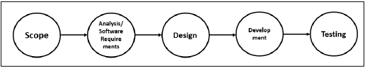
As the project completion date is based on a set of sequential tasks, these tasks are called critical tasks.
The project completion date is not based on the training, documentation and deployment. Such tasks are called non-critical tasks.
Task Dependency Relationships
Certain times, while scheduling, you may have to consider task dependency relationships. The important Task Dependency Relationships are −
- Finish-to-Start (FS)
- Finish-to-Finish (FF)
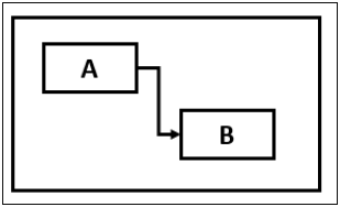
Finish-to-Start (FS)
In Finish-to-Start (FS) task dependency relationship, Task B cannot start till Task A is completed.
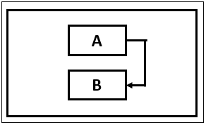
Finish-to-Finish (FF)
In Finish-to-Finish (FF) task dependency relationship, Task B cannot finish till Task A is completed.
Gantt Chart
A Gantt chart is a type of bar chart, adapted by Karol Adamiecki in 1896 and independently by Henry Gantt in the 1910s, that illustrates a project schedule. Gantt charts illustrate the start and finish dates of the terminal elements and summary elements of a project.
You can take the Outline Format in Figure 2 into Microsoft Project to obtain a Gantt Chart View.
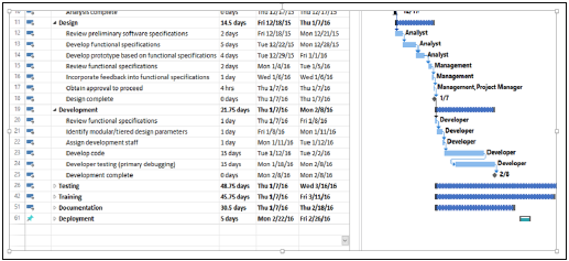
Milestones
Milestones are the critical stages in your schedule. They will have a duration of zero and are used to flag that you have completed certain set of tasks. Milestones are usually shown as a diamond.
For example, in the above Gantt Chart, Design Complete and Development Complete are shown as milestones, represented with a diamond shape.
Milestones can be tied to Contract Terms.
Advantages of Estimation using WBS
WBS simplifies the process of project estimation to a great extent. It offers the following advantages over other estimation techniques −
In WBS, the entire work to be done by the project is identified. Hence, by reviewing the WBS with project stakeholders, you will be less likely to omit any work needed to deliver the desired project deliverables.
WBS results in more accurate cost and schedule estimates.
The project manager obtains team participation to finalize the WBS. This involvement of the team generates enthusiasm and responsibility in the project.
WBS provides a basis for task assignments. As a precise task is allocated to a particular team member who would be accountable for its accomplishment.
WBS enables monitoring and controlling at task level. This allows you to measure progress and ensure that your project will be delivered on time.
Estimation Techniques - Planning Poker
Planning Poker Estimation
Planning Poker is a consensus-based technique for estimating, mostly used to estimate effort or relative size of user stories in Scrum.
Planning Poker combines three estimation techniques − Wideband Delphi Technique, Analogous Estimation, and Estimation using WBS.
Planning Poker was first defined and named by James Grenning in 2002 and later popularized by Mike Cohn in his book "Agile Estimating and Planning, whose company trade marked the term.
Planning Poker Estimation Technique
In Planning Poker Estimation Technique, estimates for the user stories are derived by playing planning poker. The entire Scrum team is involved and it results in quick but reliable estimates.
Planning Poker is played with a deck of cards. As Fibonacci sequence is used, the cards have numbers - 1, 2, 3, 5, 8, 13, 21, 34, etc. These numbers represent the Story Points. Each estimator has a deck of cards. The numbers on the cards should be large enough to be visible to all the team members, when one of the team members holds up a card.
One of the team members is selected as the Moderator. The moderator reads the description of the user story for which estimation is being made. If the estimators have any questions, product owner answers them.
Each estimator privately selects a card representing his or her estimate. Cards are not shown until all the estimators have made a selection. At that time, all cards are simultaneously turned over and held up so that all team members can see each estimate.
In the first round, it is very likely that the estimations vary. The high and low estimators explain the reason for their estimates. Care should be taken that all the discussions are meant for understanding only and nothing is to be taken personally. The moderator has to ensure the same.
The team can discuss the story and their estimates for a few more minutes.
The moderator can take notes on the discussion that will be helpful when the specific story is developed. After the discussion, each estimator re-estimates by again selecting a card. Cards are once again kept private until everyone has estimated, at which point they are turned over at the same time.
Repeat the process till the estimates converge to a single estimate that can be used for the story. The number of rounds of estimation may vary from one user story to another.
Benefits of Planning Poker Estimation
Planning poker combines three methods of estimation −
Expert Opinion − In expert opinion-based estimation approach, an expert is asked how long something will take or how big it will be. The expert provides an estimate relying on his or her experience or intuition or gut feel. Expert Opinion Estimation usually doesnt take much time and is more accurate compared to some of the analytical methods.
Analogy − Analogy estimation uses comparison of user stories. The user story under estimation is compared with similar user stories implemented earlier, giving accurate results as the estimation is based on proven data.
Disaggregation − Disaggregation estimation is done by splitting a user story into smaller, easier-to-estimate user stories. The user stories to be included in a sprint are normally in the range of two to five days to develop. Hence, the user stories that possibly take longer duration need to be split into smaller use-Cases. This approach also ensures that there would be many stories that are comparable.
Estimation Techniques - Testing
Test efforts are not based on any definitive timeframe. The efforts continue until some pre-decided timeline is set, irrespective of the completion of testing.
This is mostly due to the fact that conventionally, test effort estimation is a part of the development estimation. Only in the case of estimation techniques that use WBS, such as Wideband Delphi, Three-point Estimation, PERT, and WBS, you can obtain the values for the estimates of the testing activities.
If you have obtained the estimates as Function Points (FP), then as per Caper Jones,
Number of Test Cases = (Number of Function Points) × 1.2
Once you have the number of test cases, you can take productivity data from organizational database and arrive at the effort required for testing.
Percentage of Development Effort Method
Test effort required is a direct proportionate or percentage of the development effort. Development effort can be estimated using Lines of Code (LOC) or Function Points (FP). Then, the percentage of effort for testing is obtained from Organization Database. The percentage so obtained is used to arrive at the effort estimate for testing.
Estimating Testing Projects
Several organizations are now providing independent verification and validation services to their clients and that would mean the project activities would entirely be testing activities.
Estimating testing projects requires experience on varied projects for the software test life cycle. When you are estimating a testing project, consider −
- Team skills
- Domain Knowledge
- Complexity of the application
- Historical data
- Bug cycles for the project
- Resources availability
- Productivity variations
- System environment and downtime
Testing Estimation Techniques
The following testing estimation techniques are proven to be accurate and are widely used −
- PERT software testing estimation technique
- UCP Method
- WBS
- Wideband Delphi technique
- Function point/Testing point analysis
- Percentage distribution
- Experience-based testing estimation technique
PERT Software Testing Estimation Technique
PERT software testing estimation technique is based on statistical methods in which each testing task is broken down into sub-tasks and then three types of estimation are done on each sub-tasks.
The formula used by this technique is −
Test Estimate = (O + (4 × M) + E)/6
Where,
O = Optimistic estimate (best case scenario in which nothing goes wrong and all conditions are optimal).
M = Most likely estimate (most likely duration and there may be some problem but most of the things will go right).
L = Pessimistic estimate (worst case scenario where everything goes wrong).
Standard Deviation for the technique is calculated as −
Standard Deviation (SD) = (E − O)/6
Use-Case Point Method
UCP Method is based on the use cases where we calculate the unadjusted actor weights and unadjusted use case weights to determine the software testing estimation.
Use-case is a document which specifies different users, systems or other stakeholders interacting with the concerned application. They are named as Actors. The interactions accomplish some defined goals protecting the interest of all stakeholders through different behavior or flow termed as scenarios.
Step 1 − Count the no. of actors. Actors include positive, negative and exceptional.
Step 2 − Calculate unadjusted actor weights as
Unadjusted Actor Weights = Total no. of Actors
Step 3 − Count the number of use-cases.
Step 4 − Calculate unadjusted use-case weights as
Unadjusted Use-Case Weights = Total no. of Use-Cases
Step 5 − Calculate unadjusted use-case points as
Unadjusted Use-Case Points = (Unadjusted Actor Weights + Unadjusted Use-Case Weights)
Step 6 − Determine the technical/environmental factor (TEF). If unavailable, take it as 0.50.
Step 7 − Calculate adjusted use-case point as
Adjusted Use-Case Point = Unadjusted Use-Case Points × [0.65 + (0.01 × TEF]
Step 8 − Calculate total effort as
Total Effort = Adjusted Use-Case Point × 2
Work Breakdown Structure
Step 1 − Create WBS by breaking down the test project into small pieces.
Step 2 − Divide modules into sub-modules.
Step 3 Divide sub-modules further into functionalities.
Step 4 − Divide functionalities into sub-functionalities.
Step 5 − Review all the testing requirements to make sure they are added in WBS.
Step 6 − Figure out the number of tasks your team needs to complete.
Step 7 − Estimate the effort for each task.
Step 8 − Estimate the duration of each task.
Wideband Delphi Technique
In Wideband Delphi Method, WBS is distributed to a team comprising of 3-7 members for re-estimating the tasks. The final estimate is the result of the summarized estimates based on the team consensus.
This method speaks more on experience rather than any statistical formula. This method was popularized by Barry Boehm to emphasize on the group iteration to reach a consensus where the team visualized different aspects of the problems while estimating the test effort.
Function Point / Testing Point Analysis
FPs indicate the functionality of software application from the user's perspective and is used as a technique to estimate the size of a software project.
In testing, estimation is based on requirement specification document, or on a previously created prototype of the application. To calculate FP for a project, some major components are required. They are −
Unadjusted Data Function Points − i) Internal Files, ii) External Interfaces
Unadjusted Transaction Function Points − i) User Inputs, ii) User Outputs & iii) User Inquiries
Capers Jones basic formula −
Number of Test Cases = (Number of Function Points) × 1.2
Total Actual Effort (TAE) −
(Number of Test cases) × (Percentage of Development Effort /100)
Percentage Distribution
In this technique, all the phases of Software Development Life Cycle (SDLC) are assigned effort in %. This can be based on past data from similar projects. For example −
| Phase | % of Effort |
|---|---|
| Project Management | 7% |
| Requirements | 9% |
| Design | 16% |
| Coding | 26% |
| Testing (all Test Phases) | 27% |
| Documentation | 9% |
| Installation and Training | 6% |
Next, % of effort for testing (all test phases) is further distributed for all Testing Phases −
| All Testing Phases | % of Effort |
|---|---|
| Component Testing | 16 |
| Independent Testing | 84 |
| Total | 100 |
| Independent Testing | % of Effort |
|---|---|
| Integration Testing | 24 |
| System Testing | 52 |
| Acceptance Testing | 24 |
| Total | 100 |
| System Testing | % of Effort |
|---|---|
| Functional System Testing | 65 |
| Non-functional System Testing | 35 |
| Total | 100 |
| Test Planning and Design Architecture | 50% |
| Review phase | 50% |
Experience-based Testing Estimation Technique
This technique is based on analogies and experts. The technique assumes that you already tested similar applications in previous projects and collected metrics from those projects. You also collected metrics from previous tests. Take inputs from subject matter experts who know the application (as well as testing) very well and use the metrics you have collected and arrive at the testing effort.