- Signals & Systems Home
- Signals & Systems Overview
- Introduction
- Signals Basic Types
- Signals Classification
- Signals Basic Operations
- Systems Classification
- Types of Signals
- Representation of a Discrete Time Signal
- Continuous-Time Vs Discrete-Time Sinusoidal Signal
- Even and Odd Signals
- Properties of Even and Odd Signals
- Periodic and Aperiodic Signals
- Unit Step Signal
- Unit Ramp Signal
- Unit Parabolic Signal
- Energy Spectral Density
- Unit Impulse Signal
- Power Spectral Density
- Properties of Discrete Time Unit Impulse Signal
- Real and Complex Exponential Signals
- Addition and Subtraction of Signals
- Amplitude Scaling of Signals
- Multiplication of Signals
- Time Scaling of Signals
- Time Shifting Operation on Signals
- Time Reversal Operation on Signals
- Even and Odd Components of a Signal
- Energy and Power Signals
- Power of an Energy Signal over Infinite Time
- Energy of a Power Signal over Infinite Time
- Causal, Non-Causal, and Anti-Causal Signals
- Rectangular, Triangular, Signum, Sinc, and Gaussian Functions
- Signals Analysis
- Types of Systems
- What is a Linear System?
- Time Variant and Time-Invariant Systems
- Linear and Non-Linear Systems
- Static and Dynamic System
- Causal and Non-Causal System
- Stable and Unstable System
- Invertible and Non-Invertible Systems
- Linear Time-Invariant Systems
- Transfer Function of LTI System
- Properties of LTI Systems
- Response of LTI System
- Fourier Series
- Fourier Series
- Fourier Series Representation of Periodic Signals
- Fourier Series Types
- Trigonometric Fourier Series Coefficients
- Exponential Fourier Series Coefficients
- Complex Exponential Fourier Series
- Relation between Trigonometric & Exponential Fourier Series
- Fourier Series Properties
- Properties of Continuous-Time Fourier Series
- Time Differentiation and Integration Properties of Continuous-Time Fourier Series
- Time Shifting, Time Reversal, and Time Scaling Properties of Continuous-Time Fourier Series
- Linearity and Conjugation Property of Continuous-Time Fourier Series
- Multiplication or Modulation Property of Continuous-Time Fourier Series
- Convolution Property of Continuous-Time Fourier Series
- Convolution Property of Fourier Transform
- Parseval’s Theorem in Continuous Time Fourier Series
- Average Power Calculations of Periodic Functions Using Fourier Series
- GIBBS Phenomenon for Fourier Series
- Fourier Cosine Series
- Trigonometric Fourier Series
- Derivation of Fourier Transform from Fourier Series
- Difference between Fourier Series and Fourier Transform
- Wave Symmetry
- Even Symmetry
- Odd Symmetry
- Half Wave Symmetry
- Quarter Wave Symmetry
- Fourier Transform
- Fourier Transforms
- Fourier Transforms Properties
- Fourier Transform – Representation and Condition for Existence
- Properties of Continuous-Time Fourier Transform
- Table of Fourier Transform Pairs
- Linearity and Frequency Shifting Property of Fourier Transform
- Modulation Property of Fourier Transform
- Time-Shifting Property of Fourier Transform
- Time-Reversal Property of Fourier Transform
- Time Scaling Property of Fourier Transform
- Time Differentiation Property of Fourier Transform
- Time Integration Property of Fourier Transform
- Frequency Derivative Property of Fourier Transform
- Parseval’s Theorem & Parseval’s Identity of Fourier Transform
- Fourier Transform of Complex and Real Functions
- Fourier Transform of a Gaussian Signal
- Fourier Transform of a Triangular Pulse
- Fourier Transform of Rectangular Function
- Fourier Transform of Signum Function
- Fourier Transform of Unit Impulse Function
- Fourier Transform of Unit Step Function
- Fourier Transform of Single-Sided Real Exponential Functions
- Fourier Transform of Two-Sided Real Exponential Functions
- Fourier Transform of the Sine and Cosine Functions
- Fourier Transform of Periodic Signals
- Conjugation and Autocorrelation Property of Fourier Transform
- Duality Property of Fourier Transform
- Analysis of LTI System with Fourier Transform
- Relation between Discrete-Time Fourier Transform and Z Transform
- Convolution and Correlation
- Convolution in Signals and Systems
- Convolution and Correlation
- Correlation in Signals and Systems
- System Bandwidth vs Signal Bandwidth
- Time Convolution Theorem
- Frequency Convolution Theorem
- Energy Spectral Density and Autocorrelation Function
- Autocorrelation Function of a Signal
- Cross Correlation Function and its Properties
- Detection of Periodic Signals in the Presence of Noise (by Autocorrelation)
- Detection of Periodic Signals in the Presence of Noise (by Cross-Correlation)
- Autocorrelation Function and its Properties
- PSD and Autocorrelation Function
- Sampling
- Signals Sampling Theorem
- Nyquist Rate and Nyquist Interval
- Signals Sampling Techniques
- Effects of Undersampling (Aliasing) and Anti Aliasing Filter
- Different Types of Sampling Techniques
- Laplace Transform
- Laplace Transforms
- Common Laplace Transform Pairs
- Laplace Transform of Unit Impulse Function and Unit Step Function
- Laplace Transform of Sine and Cosine Functions
- Laplace Transform of Real Exponential and Complex Exponential Functions
- Laplace Transform of Ramp Function and Parabolic Function
- Laplace Transform of Damped Sine and Cosine Functions
- Laplace Transform of Damped Hyperbolic Sine and Cosine Functions
- Laplace Transform of Periodic Functions
- Laplace Transform of Rectifier Function
- Laplace Transforms Properties
- Linearity Property of Laplace Transform
- Time Shifting Property of Laplace Transform
- Time Scaling and Frequency Shifting Properties of Laplace Transform
- Time Differentiation Property of Laplace Transform
- Time Integration Property of Laplace Transform
- Time Convolution and Multiplication Properties of Laplace Transform
- Initial Value Theorem of Laplace Transform
- Final Value Theorem of Laplace Transform
- Parseval's Theorem for Laplace Transform
- Laplace Transform and Region of Convergence for right sided and left sided signals
- Laplace Transform and Region of Convergence of Two Sided and Finite Duration Signals
- Circuit Analysis with Laplace Transform
- Step Response and Impulse Response of Series RL Circuit using Laplace Transform
- Step Response and Impulse Response of Series RC Circuit using Laplace Transform
- Step Response of Series RLC Circuit using Laplace Transform
- Solving Differential Equations with Laplace Transform
- Difference between Laplace Transform and Fourier Transform
- Difference between Z Transform and Laplace Transform
- Relation between Laplace Transform and Z-Transform
- Relation between Laplace Transform and Fourier Transform
- Laplace Transform – Time Reversal, Conjugation, and Conjugate Symmetry Properties
- Laplace Transform – Differentiation in s Domain
- Laplace Transform – Conditions for Existence, Region of Convergence, Merits & Demerits
- Z Transform
- Z-Transforms (ZT)
- Common Z-Transform Pairs
- Z-Transform of Unit Impulse, Unit Step, and Unit Ramp Functions
- Z-Transform of Sine and Cosine Signals
- Z-Transform of Exponential Functions
- Z-Transforms Properties
- Properties of ROC of the Z-Transform
- Z-Transform and ROC of Finite Duration Sequences
- Conjugation and Accumulation Properties of Z-Transform
- Time Shifting Property of Z Transform
- Time Reversal Property of Z Transform
- Time Expansion Property of Z Transform
- Differentiation in z Domain Property of Z Transform
- Initial Value Theorem of Z-Transform
- Final Value Theorem of Z Transform
- Solution of Difference Equations Using Z Transform
- Long Division Method to Find Inverse Z Transform
- Partial Fraction Expansion Method for Inverse Z-Transform
- What is Inverse Z Transform?
- Inverse Z-Transform by Convolution Method
- Transform Analysis of LTI Systems using Z-Transform
- Convolution Property of Z Transform
- Correlation Property of Z Transform
- Multiplication by Exponential Sequence Property of Z Transform
- Multiplication Property of Z Transform
- Residue Method to Calculate Inverse Z Transform
- System Realization
- Cascade Form Realization of Continuous-Time Systems
- Direct Form-I Realization of Continuous-Time Systems
- Direct Form-II Realization of Continuous-Time Systems
- Parallel Form Realization of Continuous-Time Systems
- Causality and Paley Wiener Criterion for Physical Realization
- Discrete Fourier Transform
- Discrete-Time Fourier Transform
- Properties of Discrete Time Fourier Transform
- Linearity, Periodicity, and Symmetry Properties of Discrete-Time Fourier Transform
- Time Shifting and Frequency Shifting Properties of Discrete Time Fourier Transform
- Inverse Discrete-Time Fourier Transform
- Time Convolution and Frequency Convolution Properties of Discrete-Time Fourier Transform
- Differentiation in Frequency Domain Property of Discrete Time Fourier Transform
- Parseval’s Power Theorem
- Miscellaneous Concepts
- What is Mean Square Error?
- What is Fourier Spectrum?
- Region of Convergence
- Hilbert Transform
- Properties of Hilbert Transform
- Symmetric Impulse Response of Linear-Phase System
- Filter Characteristics of Linear Systems
- Characteristics of an Ideal Filter (LPF, HPF, BPF, and BRF)
- Zero Order Hold and its Transfer Function
- What is Ideal Reconstruction Filter?
- What is the Frequency Response of Discrete Time Systems?
- Basic Elements to Construct the Block Diagram of Continuous Time Systems
- BIBO Stability Criterion
- BIBO Stability of Discrete-Time Systems
- Distortion Less Transmission
- Distortionless Transmission through a System
- Rayleigh’s Energy Theorem
What is Ideal Reconstruction Filter?
What is Data Reconstruction?
Data reconstruction is defined as the process of obtaining the analog signal $x\mathrm{\left(\mathrm{t}\right)}$ from the sampled signal $\mathrm{x_{s}(t)}$. The data reconstruction is also known as interpolation.
The sampled signal is given by,
$$\mathrm{x_{s}(t)\:=\:x(t)\sum_{n=-\infty}^{\infty}\:\delta(t\:-\:nT)}$$
$$\mathrm{\Rightarrow\: x_{s}(t)\:=\:\sum_{n=-\infty}^{\infty}\:x(nT)\delta(t \:-\: nT)}$$
Where, $\mathrm{\delta(t\:-\:nT)}$ is zero except at the instants t = nT. A reconstruction filter which is assumed to be linear and time invariant has unit impulse response $\mathrm{h(t)}$. The output of the reconstruction filter is given by the convolution as,
$$\mathrm{y(t)\:=\:\int_{-\infty}^{\infty}\:\sum_{n=-\infty}^{\infty}\:x(nT)\delta(k\:-\:nT)h(t\:-\:k)dk}$$
By rearranging the order of integration and summation, we get,
$$\mathrm{y(t)\:=\:\sum_{n=-\infty}^{\infty}\:x(nT)\int_{-\infty}^{\infty}\:\delta(k\:-\:nT)h(t\:-\:k)dk}$$
$$\mathrm{\therefore\:y(t)\:=\:\sum_{n=-\infty}^{\infty}\:x(nT)h(t\:-\:nT)}$$
Ideal Reconstruction Filter
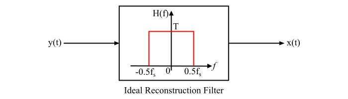
An ideal reconstruction filter is used to construct a smooth analog signal from a sampled signal. If a signal $\mathrm{x(t)}$ is sampled at a frequency greater than the Nyquist rate and the sampled signal $\mathrm{x_{s}(t)}$ is then passed through an ideal reconstruction filter (or ideal low pass filter), with bandwidth greater than $\mathrm{f_{m}}$ (which is maximum frequency present in the signal) but less than $\mathrm{(f_{s}\:-\:f_{m})}$ and a band amplitude response of T, then output of the filter is $\mathrm{x(t)}$. The bandwidth of the ideal reconstruction filter is taken equal to 0.5 $\mathrm{f_{s}}$.
Therefore, the transfer function of the ideal reconstruction filter is given by,
$$\mathrm{H(f)\:=\:\begin{cases} T \:;\: \text{ for } \:\left|f \right|\:\lt\:0.5 f_{s} \\\\ 0 \:;\: \text{ otherwise} \end{cases}}$$
The block diagram of an ideal reconstruction filter is shown in the figure.
The impulse response of the ideal reconstruction filter is given by,
$$\mathrm{h(t)\:=\:\int_{-0.5 f_{s}}^{0.5 f_{s}}T\:e^{j2\pi ft}\:df}$$
$$\mathrm{\Rightarrow\: h(t)\:=\:T\left[\frac{e^{j2\pi ft}}{j2\pi t}\right ]^{0.5 f_{s}}_{-0.5f_{s}}\:=\:\frac{T}{j2\pi t}\left(e^{j\pi f_{s}t}\:-\:e^{-j\pi f_{s}t} \right)}$$
$$\mathrm{\Rightarrow\: h(t)\:=\:\frac{1}{\pi f_{s}t}\left(\frac{e^{j\pi f_{s}t}\:-\:e^{-j\pi f_{s}t}}{2j}\right )\:=\: \frac{sin\:\pi f_{s}t}{\pi f_{s}t}}$$
$$\mathrm{\therefore\: h(t)\:=\:sinc(f_{s}t)}$$
By substituting value of the impulse response in the expression for the output of the reconstruction filter, we have,
$$\mathrm{y(t)\:=\:x(t)\:=\:\sum_{n=-\infty}^{\infty}\:x(nT)\:sinc\:f_{s}\left(t\:-\:nT \right)}$$
$$\mathrm{\therefore\: x(t)\:=\:\sum_{n=-\infty}^{\infty}\:x(nT)\:sinc\:\left ( \frac{t}{T}\:-\:n \right )}$$
Thus, it is clear that the original signal can be reconstructed by weighing each sample by a sinc function centred at the sample time and summing. The ideal reconstruction filter is non-causal and its impulse response is not limited. Therefore, it cannot be used for real-time applications.