Separating Planes In SVM

Support Vector Machine (SVM) is a supervised algorithm used widely in handwriting recognition, sentiment analysis and many more. To separate different classes, SVM calculates the optimal hyperplane that more or less accurately creates a margin between the two classes.

Here are a few ways to separate hyperplanes in SVM.

• Data Processing − SVM requires data that is normalised, scaled and centred since they are sensitive to such features.

• Choose a Kernel − A kernel function is used to transform the input into a higher dimensional space. Some of them include linear, polynomial and radial base functions.

Let us consider two cases where SVM hyperplanes can be differentiated. They are −

• Linearly separable case.

• Non-linearly separable case.

Example 1

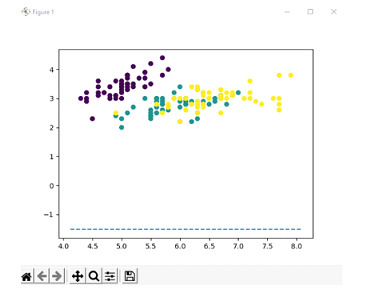
For the linearly separable case, let us consider the iris dataset of 2 dimension features. A linearly separable case is when the features can be separated by a hyperplane linearly. The iris dataset is a good beginner-friendly way in order to depict hyperplanes that are linearly separable. The goal is to display a hyperplane that is linear in nature.

Algorithm

• Import all the libraries

• Load the Iris dataset and assign the data and target features to variables x and y respectively.

• Using the train_test_split function, assign values to x_train, x_test, y_train, and y_test.

• Build the SVM model with a linear kernel and fit the model concerning the training data points.

• Predict the labels and print the accuracy of the model.

• Using the model assign the weight and bias of the model as the coefficient of the model and intercept of the line respectively.

• Using weight and bias, calculate the slope and y_intercept.

• Plot the data points in a graph and showcase it.

from sklearn import datasets
from sklearn.svm import SVC
from sklearn.model_selection import train_test_split as tts
from sklearn.metrics import accuracy_score
import matplotlib.pyplot as plt
import numpy as np

iris=datasets.load_iris()
x=iris.data
y=iris.target

x_train, x_test, y_train, y_test = tts(x,y,test_size=0.3,random_state=10)

#build an SVM model with linear kernel
clf=SVC(kernel='linear')

#fit the model
clf.fit(x_train,y_train)

#predict the labels
y_pred=clf.predict(x_test)

#calculate the accuracy
acc=accuracy_score(y_test,y_pred)
print("Accuracy: ", acc)

#get the hyperplane parameters
w=clf.coef_[0]
b=clf.intercept_[0]

#calculate the slope and intercept
slope = -w[0]/w[1]
y_int = -b/w[1]

#plot the dataset and hyperplane
plt.scatter(x[:,0], x[:,1], c=y)
axes=plt.gca()
x_vals=np.array(axes.get_xlim())
y_vals=y_int+slope*x_vals
plt.plot(x_vals, y_vals, '--')
plt.show()

We split the dataset into training and testing sets where the testing set is 30% of the total data. We then create an SVM classifier with a linear kernel and fit the model to the training data.

We predict the labels for testing data and store the result thus obtained in a separate variable and calculate the accuracy of the model by comparing the predicted values with that of true values and print the accuracy thus obtained which is 1.0.

Then the parameters of the hyperplane are retrieved from trained dataset and calculate the slope and intercept of the hyperplane which is then plotted using scatter plot with different colors for each category.

Accuracy: 1.0

Output

Example 2

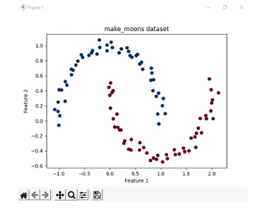
Consider an example where the cases are not linearly separable. In this case, we use the make_moons dataset available in the scikit-learn library. The make_moons dataset is a good way to depict when 2 or more classes are not linearly separable. Hence, this example is used to depict a non-linear separable case.

Let us first print the data points of the dataset to have an idea of what we’re working with.

Algorithm

• Import all necessary libraries.

• Generate the make_moons dataset with 100 samples with a minimal noise level.

• Plot these data points in a graph and print and assign the colourmap as red and blue.

import matplotlib.pyplot as plt
from sklearn.datasets import make_moons

# Generate the make_moons dataset with 100 samples and a noise level of 0.05
X, y = make_moons(n_samples=100, noise=0.05, random_state=42)

# To show the dataset
plt.scatter(X[:, 0], X[:, 1], c=y, cmap=plt.cm.RdBu_r)

# Set the plot labels and title
plt.xlabel('Feature 1')
plt.ylabel('Feature 2')
plt.title('make_moons dataset')

# Show the plot
plt.show()

Output

Algorithm

• Import all the libraries used in the program

• Generate 100 data samples from the make_moons dataset with noise as low as possible.

• Initialize an SVC classifier with radial basis function (RBF) kernel and train the data points based on the classifier.

• According to the data points, fit the classifier initialized earlier to the dataset

• Find the maximum and minimum points of the features and labels in the data.

• Using the above values, construct a mesh grid using linspace function.

• To return a one-dimensional representation of the mesh grid, the ravel function is applied and sliced along the second axis using np.c_

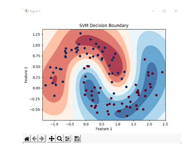
• To define the decision boundary, create a contour plot of the decision boundary.

• Print the image and labels.

Example

import numpy as np
import matplotlib.pyplot as plt
from sklearn import datasets
from sklearn.svm import SVC

# load moons dataset
x, y = datasets.make_moons(n_samples=100, noise=0.15, random_state=42)

# create an SVM classifier implementing RBF kernel
clf = SVC(kernel='rbf', gamma=2)

# train the classifier on the dataset
clf.fit(X, y)

# create a meshgrid representing features and labels
x_min, x_max = x[:, 0].min() - 0.1, x[:, 0].max() + 0.1
y_min, y_max = x[:, 1].min() - 0.1, x[:, 1].max() + 0.1
xx, yy = np.meshgrid(np.linspace(x_min, x_max, 500), np.linspace(y_min, y_max, 500))
z = clf.decision_function(np.c_[xx.ravel(), yy.ravel()])
z = z.reshape(xx.shape)

# create a contour plot of the decision boundary
plt.contourf(xx, yy, z, cmap=plt.cm.RdBu, alpha=0.8)
plt.scatter(x[:, 0], x[:, 1], c=y, cmap=plt.cm.RdBu_r)

# set the plot labels and title
plt.xlabel('Feature 1')
plt.ylabel('Feature 2')
plt.title('SVM Decision Boundary')

# show the plot
plt.show()

We generate the dataset by creating 100 samples with a noise level of 0.15 and random seed of 42 and create an SVM classifier and train the classifier on the dataset. We then define a set of points to represent the features and labels. We then calculate decision function values for those points and reshape them to match the dimensions of the grid. We then create a contour plot of the decision boundary where the decision function values determine the colour of the regions. We also plot the original data points with different colours representing different categories.

Output

Conclusion

Support Vector Machine is one of the more widely used algorithms used for a variety of domains, mainly text and speech classification, or sentiment analysis in NLP. Its versatile nature in the case of classification makes it one of the more popular algorithms.

In other cases, it has its own drawbacks. Sometimes, SVM can be very computationally intensive and the data fed to the model needs to be checked carefully due to the sensitivity of the model.